The Generalized Brillouin Zone and Non-Bloch Band Theory

In a non-Hermitian chain with the skin effect, the open-chain eigenstates are not Bloch waves \(\beta^n\) with \(|\beta| = |e^{ik}| = 1\), but decay as \(|\beta|^n\) with \(|\beta| \neq 1\). Yao and Wang (2018) put the open-chain bands on a generalized Brillouin zone (GBZ), the loop in the complex \(\beta\) plane on which \(H(\beta) = \sum_n t(n)\beta^n\) reproduces them, and Yokomizo and Murakami (2019) showed how to construct it for any 1D model: sort the roots of \(\det[H(\beta) - E] = 0\) by modulus; \(E\) belongs to the open-chain spectrum when the middle two have equal moduli.

For the non-Hermitian SSH chain of Yao and Wang – intracell hoppings \(t_1 \pm \gamma/2\) to the right and to the left, intercell \(t_2\) – the GBZ is the circle \(|\beta| = r = \sqrt{|(t_1 - \gamma/2)/(t_1 + \gamma/2)|}\). The Bloch Hamiltonian then predicts the wrong phase diagram: its spectrum closes its gap at \(t_1 = t_2 \pm \gamma/2\), and its winding number is a meaningless \(1/2\) in between, while the open chain changes phase at \(t_1^2 = t_2^2 + \gamma^2/4\). The winding number of the non-Bloch Hamiltonian along the GBZ restores the bulk-boundary correspondence: it is 1 exactly when the open chain has zero modes. gbz() and get_ham_beta() compute both.

import numpy as np
import matplotlib.pyplot as plt

import tbkit.lattices as lattices
from tbkit.bridges import finite_system
from tbkit.lattice import Lattice
from tbkit.kspace import KSpace
from tbkit.plot import Plot

The Hatano-Nelson chain: a circle of radius sqrt(t_L / t_R)

t_right, t_left = 1., 0.5
hn = KSpace(lattices.chain())
hn.set_hopping([{'i': 0, 'j': 0, 'R': (1,), 't': t_right},
                        {'i': 0, 'j': 0, 'R': (-1,), 't': t_left}], hermitian=False)

Ten sites of the Hatano-Nelson chain (finite_system()): one site per cell and nearest-neighbour bonds, non-reciprocal – each carries \(t_R\) one way and \(t_L\) the other. The widths drawn are those of \(t_R\).

fig_lat = Plot(finite_system(hn, 10)).lattice(plt_hop=True, ms=12, figsize=(7, 1.2))

The open chain’s spectrum, and the GBZ it lies on:

en_hn = np.linalg.eigvals(hn.finite_ham(60))
beta_hn = hn.gbz(en_hn)
print('Hatano-Nelson: |beta| on the GBZ = {:.6f}, sqrt(t_L/t_R) = {:.6f}'
          .format(np.abs(beta_hn).mean(), np.sqrt(t_left / t_right)))
assert np.allclose(np.abs(beta_hn), np.sqrt(t_left / t_right))
# the open-chain spectrum is H(beta) on it
for e, b in zip(en_hn[:10], beta_hn[:10, 0]):
    assert np.isclose(hn.get_ham_beta(b)[0, 0], e)

Hatano-Nelson: |beta| on the GBZ = 0.707107, sqrt(t_L/t_R) = 0.707107

The non-Hermitian SSH chain

t2, gamma = 1., 4 / 3
lat = Lattice(unit_cell=[{'tag': 'a', 'r0': (0., 0.)}, {'tag': 'b', 'r0': (0.5, 0.)}], prim_vec=[(1., 0.)])


def nh_ssh(t1):
    ks = KSpace(lat)
    ks.set_hopping([{'i': 0, 'j': 1, 'R': (0,), 't': t1 + gamma / 2},
                            {'i': 1, 'j': 0, 'R': (0,), 't': t1 - gamma / 2},
                            {'i': 1, 'j': 0, 'R': (1,), 't': t2},
                            {'i': 0, 'j': 1, 'R': (-1,), 't': t2}], hermitian=False)
    return ks


def radius(t1):
    return np.sqrt(abs((t1 - gamma / 2) / (t1 + gamma / 2)))

Eight cells of the chain (finite_system()), orbitals a and b in two colours, bond widths proportional to the amplitudes: \(t_1 + \gamma/2\) inside each cell (the reverse intra-cell hopping is \(t_1 - \gamma/2\), not drawn) and \(t_2\) between cells, here for \(t_1 = 1.1\).

fig_ssh = Plot(finite_system(nh_ssh(1.1), 8)).lattice(plt_hop=True, ms=7, c=2.5, figsize=(7, 1.2))

The winding number on the GBZ and on the Brillouin zone:

def winding(ks, r, n=200):
    r'''(w[H_ab] - w[H_ba]) / 2 along the circle |beta| = r: the winding number
    of the chiral (off-diagonal) blocks, the Bloch one for r = 1.'''
    betas = r * np.exp(2j * np.pi * np.arange(n + 1) / n)
    hams = np.array([ks.get_ham_beta(b) for b in betas])
    w_ab, w_ba = (np.sum(np.angle(h[1:] / h[:-1])) / (2 * np.pi) for h in (hams[:, 0, 1], hams[:, 1, 0]))
    return (w_ba - w_ab) / 2


t1 = 1.1
model = nh_ssh(t1)
n_cells = 40
en, vec = np.linalg.eig(model.finite_ham(n_cells))
bulk = np.argsort(np.abs(en))[2:]  # the two zero modes are not on the GBZ
beta = model.gbz(en[bulk])
print('t1 = {}: |beta| on the GBZ = {:.6f}, r = {:.6f}'.format(t1, np.abs(beta).mean(), radius(t1)))
assert np.allclose(np.abs(beta), radius(t1), atol=1e-6)
for e, b in zip(en[bulk][:10], beta[:10, 0]):
    assert np.min(np.abs(np.linalg.eigvals(model.get_ham_beta(b)) - e)) < 1e-8
ring = np.linalg.eigvals(model.finite_ham(n_cells, periodic=True))
print('Open-chain spectrum real (max |Im E| = {:.1e}); the ring spectrum is not (max |Im E| = {:.2f}).'
          .format(np.max(np.abs(en.imag)), np.max(np.abs(ring.imag))))
assert np.max(np.abs(en.imag)) < 1e-8 and np.max(np.abs(ring.imag)) > 0.1

t1 = 1.1: |beta| on the GBZ = 0.495261, r = 0.495261
Open-chain spectrum real (max |Im E| = 8.9e-11); the ring spectrum is not (max |Im E| = 0.66).

The phase diagram: Bloch versus non-Bloch

The open-chain zero modes disappear at \(t_1 = \sqrt{t_2^2 + \gamma^2/4}\), not where the Bloch spectrum closes its gap, and the non-Bloch winding number follows them.

t_c = np.sqrt(t2 ** 2 + gamma ** 2 / 4)
t1s = np.linspace(0.8, 2., 61)
smallest, w_bloch, w_gbz = [], [], []
for t1_ in t1s:
    ks = nh_ssh(t1_)
    smallest.append(np.min(np.abs(np.linalg.eigvals(ks.finite_ham(n_cells)))))
    w_bloch.append(winding(ks, 1.))
    w_gbz.append(winding(ks, radius(t1_)))
smallest, w_bloch, w_gbz = np.array(smallest), np.array(w_bloch), np.array(w_gbz)
inside, outside = t1s < t_c - 0.05, t1s > t_c + 0.05
assert np.all(smallest[inside] < 1e-2) and np.all(smallest[outside] > 0.05)
assert np.allclose(w_gbz[inside], 1.) and np.allclose(w_gbz[outside], 0.)
assert np.allclose(w_bloch[t1s < t2 + gamma / 2 - 0.05], 0.5)
print('Open-chain zero modes and non-Bloch winding 1 for t1 < {:.4f}, none and 0 above; '
          'Bloch winding 1/2 up to t1 = t2 + gamma/2 = {:.4f}.'.format(t_c, t2 + gamma / 2))

fig, axes = plt.subplots(1, 3, figsize=(14, 4.2))
theta = np.linspace(0, 2 * np.pi, 200)
axes[0].plot(np.cos(theta), np.sin(theta), 'k--', lw=1, label='Brillouin zone')
axes[0].plot(beta.real.ravel(), beta.imag.ravel(), 'or', ms=3, label='GBZ, $t_1 = 1.1$')
axes[0].set_aspect('equal')
axes[0].set_xlabel(r'Re $\beta$')
axes[0].set_ylabel(r'Im $\beta$')
axes[0].legend(fontsize=8)
axes[1].plot(ring.real, ring.imag, 'ob', ms=3, label='ring')
axes[1].plot(en.real, en.imag, 'or', ms=3, label='open chain')
axes[1].set_xlabel(r'Re $E$')
axes[1].set_ylabel(r'Im $E$')
axes[1].set_title('$t_1 = 1.1$')
axes[1].legend(fontsize=8)
axes[2].plot(t1s, w_gbz, 'r', label='non-Bloch winding (GBZ)')
axes[2].plot(t1s, w_bloch, 'b--', label='Bloch winding')
axes[2].plot(t1s, np.minimum(smallest, 1.), 'k', lw=1, label=r'smallest open-chain $|E|$')
axes[2].axvline(t_c, color='r', lw=0.8, ls=':')
axes[2].axvline(t2 + gamma / 2, color='b', lw=0.8, ls=':')
axes[2].set_xlabel('$t_1$')
axes[2].legend(fontsize=8)
fig.set_layout_engine('tight')

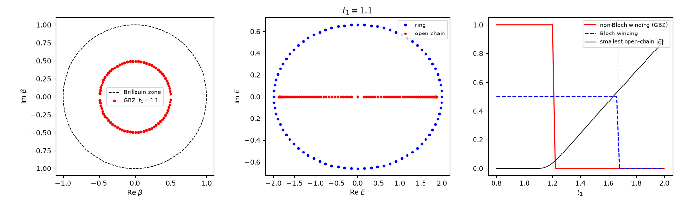
Open-chain zero modes and non-Bloch winding 1 for t1 < 1.2019, none and 0 above; Bloch winding 1/2 up to t1 = t2 + gamma/2 = 1.6667.