The Universal Absorption of Graphene: Opacity Defined by the Fine-Structure Constant

In 2008 Nair et al. held a suspended graphene membrane in front of a light source and found that one atomic layer absorbs \(\pi\alpha \approx 2.3\%\) of white light, with \(\alpha = e^2/4\pi\varepsilon_0\hbar c\) the fine-structure constant: no material parameter enters. The reason is graphene’s optical conductivity. Its massless Dirac electrons absorb at \(\hbar\omega\) through vertical transitions from \(-\hbar\omega/2\) to \(+\hbar\omega/2\), and the growing number of those transitions exactly compensates their weakening matrix elements, so

\[\mathrm{Re}\,\sigma_{xx}(\omega) = \sigma_0 = \frac{e^2}{4\hbar}\, ,\]

(spin and valleys counted) for \(2|E_F| < \hbar\omega \ll t\), as Ando, Zheng and Suzuki (2002) and Gusynin, Sharapov and Carbotte (2006) had predicted. A free-standing sheet then absorbs \(\mathrm{Re}\,\sigma/\varepsilon_0c = \pi\alpha\).

optical_conductivity() evaluates the Kubo-Greenwood formula over the Brillouin zone of the tight-binding model; joint_dos() counts the transitions.

import numpy as np
import matplotlib.pyplot as plt
from scipy.constants import alpha

import tbkit.lattices as lattices
from tbkit.bridges import finite_system
from tbkit.kspace import KSpace
from tbkit.optics import optical_conductivity, joint_dos, cell_area
from tbkit.plot import Plot


t = -1.
gra = KSpace(lattices.honeycomb())  # bond length 1
gra.set_hopping([{'i': 0, 'j': 1, 'R': R, 't': t} for R in [(0, 0), (-1, 0), (0, -1)]])

The lattice

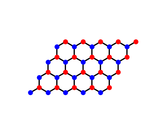
Graphene’s honeycomb lattice on a patch of \(5\times4\) cells (finite_system()): two sites per unit cell (sublattices ‘a’ and ‘b’, in two colours), each bonded to its three nearest neighbours.

fig_lat = Plot(finite_system(gra, (5, 4))).lattice(plt_hop=True, ms=12, figsize=(5.5, 4.5))

The universal conductivity

A spinless model counts each orbital once: its conductivity is half of \(\sigma_0\), i.e. \(e^2/8\hbar = \frac{\pi}{4}\frac{e^2}{h}\). At small \(\hbar\omega\) the tight-binding band adds a correction quadratic in \(\hbar\omega/t\), so the universal value is the \(\omega\to0\) limit.

sigma_0 = 2 * np.pi / 4  # e^2/(4 hbar) in units of e^2/h, two spins
omega = np.array([0.2, 0.3, 0.4])
sigma = 2 * optical_conductivity(gra, omega, e_fermi=0., eta=0.03, nk=400)
slope, limit = np.polyfit(omega ** 2, sigma.real / sigma_0, 1)
print('Re sigma(omega -> 0) = {:.4f} sigma_0'.format(limit))
assert abs(limit - 1.) < 5e-3

absorbance = limit * np.pi * alpha  # Re sigma / (epsilon_0 c)
print('absorbance of one layer: {:.2f} % (pi alpha = {:.2f} %)'.format(100 * absorbance, 100 * np.pi * alpha))
assert abs(absorbance - 0.0229) < 2e-4

Re sigma(omega -> 0) = 0.9972 sigma_0
absorbance of one layer: 2.29 % (pi alpha = 2.29 %)

Counting the transitions

The joint density of states grows linearly, \(J(\omega) = A_c\,\hbar\omega/(4\pi\hbar^2v_F^2)\) per spin with \(v_F = 3|t|a/2\). The Kubo-Greenwood weight of each transition, \(|v_{cv}|^2/\hbar\omega\) with \(|v_{cv}|^2\) of order \(v_F^2\) on a Dirac cone, falls as \(1/\omega\): the product is constant.

jdos = joint_dos(gra, omega, eta=0.02, nk=500)
slope_jdos = cell_area(gra) / (4 * np.pi * (1.5 * abs(t)) ** 2)
assert np.allclose(jdos / omega, slope_jdos, rtol=0.02)

The whole spectrum, and Pauli blocking

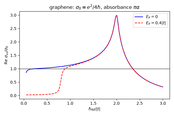
Beyond the Dirac regime, the absorption peaks at the van Hove singularity \(\hbar\omega = 2|t|\) (transitions at the M points). Doping to \(E_F\) blocks every transition below \(2|E_F|\).

w = np.linspace(0.05, 3., 120)
neutral = 2 * optical_conductivity(gra, w, e_fermi=0., eta=0.03, nk=300).real / sigma_0
doped = 2 * optical_conductivity(gra, w, e_fermi=0.4, eta=0.03, nk=300).real / sigma_0
peak = w[np.argmax(neutral)]
print('van Hove peak at hbar omega = {:.2f} |t|'.format(peak))
assert abs(peak - 2 * abs(t)) < 0.05
assert np.all(doped[w < 0.6] < 0.1) and np.allclose(doped[w > 1.6], neutral[w > 1.6], rtol=0.03)

fig, ax = plt.subplots(figsize=(6, 4))
ax.plot(w, neutral, '-b', label='$E_F = 0$')
ax.plot(w, doped, '--r', label='$E_F = 0.4|t|$')
ax.axhline(1., color='k', lw=0.8)
ax.set_xlabel(r'$\hbar\omega / |t|$')
ax.set_ylabel(r'Re $\sigma_{xx} / \sigma_0$')
ax.set_title(r'graphene: $\sigma_0 = e^2/4\hbar$, absorbance $\pi\alpha$')
ax.legend()
fig.set_layout_engine('tight')

van Hove peak at hbar omega = 2.01 |t|