Exceptional Points in Momentum Space: Encircling an EP versus a Dirac Point

A loop in the Brillouin zone around a band touching tells what kind of touching it is.

• Around a diabolical point – graphene’s Dirac point K – the two eigenvalues come back to themselves after one loop, and the eigenvector, carried along by parallel transport, comes back with a Berry phase \(\pi\): \(|u\rangle\to-|u\rangle\).

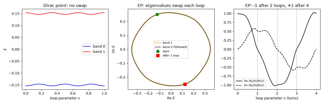
• Around a second-order exceptional point the eigenvalues are the two branches of a square root, \(E_\pm \propto \pm\sqrt{\mathbf{k}-\mathbf{k}_{EP}}\). One loop swaps the two eigenstates. A second loop brings each back, but with a sign flip: a geometric phase \(\pi\) after two turns. Only after four loops is the state fully restored. This is Heiss’s “chirality” of exceptional points, first seen by encircling an EP in the parameter space of a microwave cavity (Dembowski et al., Phys. Rev. Lett. 86, 787 (2001)).

Both are computed with tbkit.exceptional.encircle(), which follows the eigenvalue by continuation and transports the right eigenvector \(|R\rangle\) with \(\langle L|\partial R\rangle = 0\) (\(\langle L|\) the left eigenvector, \(\langle L|R\rangle = 1\)); for a Hermitian model this is the usual Berry-phase transport.

The EP is one of the pair into which \(i\gamma\sigma_x\) splits graphene’s Dirac point (see the other examples of this entry).

import numpy as np
import matplotlib.pyplot as plt

import tbkit.lattices as lattices
from tbkit.bridges import finite_system
from tbkit.kspace import KSpace
from tbkit.plot import Plot
import tbkit.exceptional as ex

NN = [{'i': 0, 'j': 1, 'R': (0, 0), 't': 1.}, {'i': 0, 'j': 1, 'R': (-1, 0), 't': 1.},
      {'i': 0, 'j': 1, 'R': (0, -1), 't': 1.}]
gamma = 0.3
graphene = KSpace(lattices.honeycomb())
graphene.set_hopping(NN)
model = KSpace(lattices.honeycomb())
model.set_hopping(NN)
model.set_hopping([{'i': 0, 'j': 1, 'R': (0, 0), 't': 1j * gamma},
                   {'i': 1, 'j': 0, 'R': (0, 0), 't': 1j * gamma}], hermitian=False)
b1, b2 = (np.array(b) for b in graphene.rec_vec_k)
K = (b1 - b2) / 3

eps = ex.find_exceptional_points(model, nk=40)
shifts = [m * b1 + n * b2 for m in (-1, 0, 1) for n in (-1, 0, 1)]
near = [(p + s, q) for p, q in zip(eps.k, eps.charge) for s in shifts
        if np.linalg.norm(p + s - K) < 0.5]
assert len(near) == 2
k_ep = near[0][0]
radius = 0.1  # the partner EP is 0.39 away: only one EP inside
assert np.linalg.norm(near[0][0] - near[1][0]) > 3 * radius

The lattice

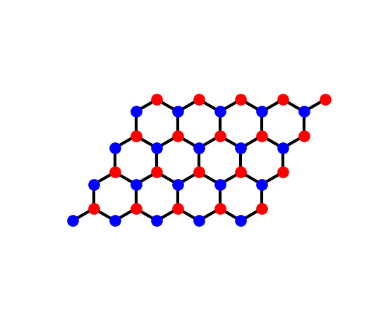
Graphene’s honeycomb lattice on a patch of \(5\times4\) cells (finite_system()): sublattices ‘a’ and ‘b’ in two colours, each bonded to its three nearest neighbours. The non-Hermitian term, \(i\gamma\) added to both directions of the intra-cell bond, adds no bond and is not drawn.

fig_lat = Plot(finite_system(graphene, (5, 4))).lattice(plt_hop=True, ms=12, figsize=(5.5, 4.5))

Around the Dirac point: one loop, Berry phase pi

dp_loop = ex.circle(K, radius)
for band in (0, 1):
    res = ex.encircle(graphene, dp_loop, band=band, n_loops=1, nk=300)
    print('Dirac point, band {}: ends on band {}, phase {:+.6f}, |overlap| {:.4f}'
          .format(band, res.final_band, res.phase, abs(res.overlap)))
    assert res.final_band == band
    assert np.isclose(abs(res.phase), np.pi, atol=1e-8)
    assert np.isclose(abs(res.overlap), 1., atol=1e-8)  # the norm is kept
dp_one = ex.encircle(graphene, dp_loop, band=0, n_loops=1, nk=300)

Dirac point, band 0: ends on band 0, phase +3.141593, |overlap| 1.0000
Dirac point, band 1: ends on band 1, phase +3.141593, |overlap| 1.0000

Around an exceptional point: swap, sign flip, return

After 1 loop the state that started on band 0 ends on band 1 – it is the other eigenvector (up to a factor). After 2 loops it is back on band 0 with a factor \(-1\); after 4 loops the factor is \(+1\). (After 1 and 3 loops the factor, \(\pm i\) here, depends on the arbitrary phase of the other band’s eigenvector at the start; after an even number of loops it is a property of the EP.)

ep_loop = ex.circle(k_ep, radius)
runs = {n: ex.encircle(model, ep_loop, band=0, n_loops=n, nk=300) for n in (1, 2, 3, 4)}
for n, res in runs.items():
    print('EP, {} loop(s): ends on band {}, factor {:+.4f}{:+.4f}i'
          .format(n, res.final_band, res.overlap.real, res.overlap.imag))
assert runs[1].final_band == 1 and runs[3].final_band == 1
assert runs[2].final_band == 0 and runs[4].final_band == 0
h0 = model.get_ham(ep_loop(0.))
v1 = runs[1].vector[-1]
assert np.allclose(h0 @ v1, runs[1].en[0, 1] * v1, atol=1e-8)  # the other eigenvector
assert np.isclose(abs(runs[2].phase), np.pi, atol=1e-8)
assert np.isclose(runs[4].phase, 0., atol=1e-8)
assert np.isclose(runs[2].overlap, -1., atol=1e-8)
assert np.isclose(runs[4].overlap, 1., atol=1e-8)

EP, 1 loop(s): ends on band 1, factor +0.0000+1.0000i
EP, 2 loop(s): ends on band 0, factor -1.0000-0.0000i
EP, 3 loop(s): ends on band 1, factor +0.0000-1.0000i
EP, 4 loop(s): ends on band 0, factor +1.0000-0.0000i

The eigenvalue swap is the vorticity 1/2, the four-loop return its double

One loop around the EP turns \(E_0 - E_1\) by \(\pi\) (vorticity \(\pm1/2\)); around the Dirac point, or around both EPs, it does not turn at all, and one loop is enough to bring both eigenvalues back.

nu_ep = ex.vorticity(model, ep_loop)
nu_dp = ex.vorticity(graphene, dp_loop)
both = ex.encircle(model, ex.circle(K, 0.35), band=0, nk=300)
print('vorticity: EP {:+.3f}, Dirac point {:+.1e}; around both EPs the state ends on band {}'
      .format(nu_ep, nu_dp, both.final_band))
assert np.isclose(abs(nu_ep), 0.5, atol=1e-10) and abs(nu_dp) < 1e-10
assert both.final_band == 0

vorticity: EP +0.500, Dirac point +7.8e-33; around both EPs the state ends on band 0

Eigenvalues along the loops

Left: around the Dirac point the two (real) eigenvalues each close on themselves. Right: around the EP, the complex eigenvalues trace one closed curve in two turns – the followed eigenvalue (dark) needs two loops to come back.

fig, axes = plt.subplots(1, 3, figsize=(13, 4.2))
axes[0].plot(dp_one.s, dp_one.en.real[:, 0], 'b', label='band 0')
axes[0].plot(dp_one.s, dp_one.en.real[:, 1], 'r', label='band 1')
axes[0].set_xlabel('loop parameter $s$')
axes[0].set_ylabel('$E$')
axes[0].set_title('Dirac point: no swap')
axes[0].legend()

two = runs[2]
axes[1].plot(two.en[:, 1].real, two.en[:, 1].imag, color='orange', lw=4, alpha=0.4, label='band 1')
axes[1].plot(two.en[:, 0].real, two.en[:, 0].imag, 'k', lw=1.2, label='band 0 (followed)')
axes[1].plot(two.en[0, 0].real, two.en[0, 0].imag, 'go', ms=8, label='start')
axes[1].plot(runs[1].en[-1, 0].real, runs[1].en[-1, 0].imag, 'rs', ms=8, label='after 1 loop')
axes[1].set_xlabel('Re $E$')
axes[1].set_ylabel('Im $E$')
axes[1].set_title('EP: eigenvalues swap each loop')
axes[1].legend(fontsize=8)

four = runs[4]
factor = [np.vdot(four.vector[0], v) / np.vdot(four.vector[0], four.vector[0]) for v in four.vector]
axes[2].plot(four.s, np.real(factor), 'k', label=r'Re $\langle R_0(0)|R(s)\rangle$')
axes[2].plot(four.s, np.imag(factor), 'k--', label=r'Im $\langle R_0(0)|R(s)\rangle$')
for n in (1, 2, 3):
    axes[2].axvline(n, color='gray', lw=0.5)
axes[2].set_xlabel('loop parameter $s$ (turns)')
axes[2].set_title('EP: -1 after 2 loops, +1 after 4')
axes[2].legend(fontsize=8)
fig.tight_layout()