Periodic Boundaries in Real Space: Tori and Cylinders

A finite flake has edges, and their states mix with the bulk ones. Wrap the sample of get_lattice() into a torus and the edges disappear: System(lat, periodic=True) measures every distance and bond angle along the shortest image, so set_hopping by neighbour order (with angles and tags) also sets the bonds that wrap around. The spectrum of an \(N_1\times N_2\) torus is then exactly that of the Bloch bands on the \(N_1\times N_2\) k-mesh. Wrapping along one vector only, periodic=(True, False), gives a cylinder, with the edge states of a ribbon.

The real-space model keeps the advantages of a System: vacancies, disorder and defects. On a torus, get_bott_index() gives the Chern number of a disordered sample.

import numpy as np
import matplotlib.pyplot as plt

import tbkit.lattices as lattices
from tbkit.kspace import KSpace
from tbkit.plot import Plot
from tbkit.system import System

t2 = 0.2


def haldane_system(n1, n2, periodic):
    lat = lattices.honeycomb()
    lat.get_lattice(n1, n2)
    sys = System(lat, periodic=periodic)
    sys.set_hopping([{'n': 1, 't': 1.}])
    # +i t2 along a2, -a1, a1 - a2 on 'a' (angles 60, 180, -60), the opposite on 'b'
    for tag, sign in (('aa', 1), ('bb', -1)):
        sys.set_hopping([{'n': 2, 'ang': 60., 'tag': tag, 't': 1j*t2*sign},
                                {'n': 2, 'ang': 0., 'tag': tag, 't': -1j*t2*sign},
                                {'n': 2, 'ang': 120., 'tag': tag, 't': -1j*t2*sign}])
    sys.set_onsite({'a': 0., 'b': 0.})
    return sys


hal = KSpace(lattices.honeycomb())
hal.set_hopping([{'i': 0, 'j': 1, 'R': R, 't': 1.} for R in [(0, 0), (-1, 0), (0, -1)]])
for R in [(0, 1), (-1, 0), (1, -1)]:
    hal.set_hopping([{'i': 0, 'j': 0, 'R': R, 't': 1j*t2}, {'i': 1, 'j': 1, 'R': R, 't': -1j*t2}])

The lattice

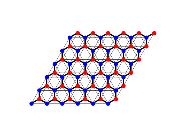
The Haldane model on a \(6\times6\)-cell flake, bond widths proportional to the amplitudes: the honeycomb lattice’s two sublattices (‘a’ and ‘b’, in two colours), the nearest-neighbour hopping (thick) and the second-neighbour hoppings \(\pm it_2\) (thin). The torus and the cylinder below add the bonds across the boundaries, which are not drawn.

fig_lat = Plot(haldane_system(6, 6, False)).lattice(plt_hop=True, ms=10, figsize=(6, 4.5))

Torus, cylinder and flake

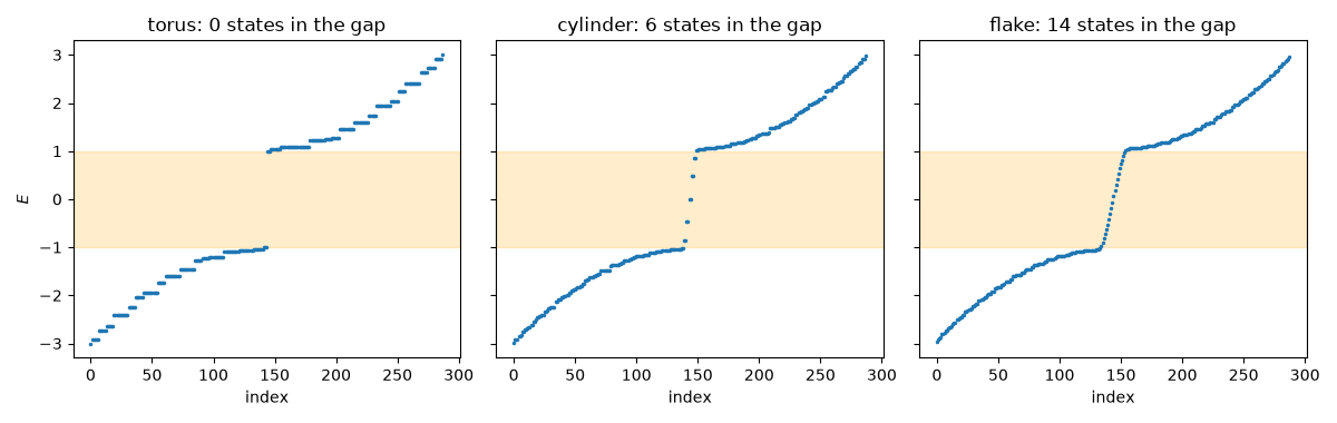
The torus has the spectrum of the k-mesh, and an empty gap. The cylinder and the flake fill the gap with the chiral edge states of the Haldane model.

n = 12
spectra = {}
for name, periodic in (('torus', True), ('cylinder', (True, False)), ('flake', False)):
    sys = haldane_system(n, n, periodic)
    sys.get_ham()
    sys.get_eig()
    spectra[name] = np.sort(sys.en.real)
mesh = np.sort(hal.mesh_bands((n, n)).ravel())
assert np.allclose(spectra['torus'], mesh, atol=1e-12)
gap = np.min(hal.mesh_bands(60)[:, 1] - hal.mesh_bands(60)[:, 0]) / 2
in_gap = {name: int(np.sum(np.abs(en) < 0.8 * gap)) for name, en in spectra.items()}
print('States inside the bulk gap:', in_gap)
assert in_gap['torus'] == 0 and in_gap['cylinder'] > 0 and in_gap['flake'] > 0

States inside the bulk gap: {'torus': 0, 'cylinder': 6, 'flake': 14}

A disordered torus keeps its Chern number

Random onsite energies and 5% vacancies: no Brillouin zone, yet the Bott index of the torus is still 1.

rng = np.random.default_rng(1)
lat = lattices.honeycomb()
lat.get_lattice(n, n)
lat.remove_sites([int(i) for i in rng.choice(lat.sites, size=int(0.05 * lat.sites), replace=False)])
dirty = System(lat, periodic=True)
dirty.set_hopping([{'n': 1, 't': 1.}])
for tag, sign in (('aa', 1), ('bb', -1)):
    dirty.set_hopping([{'n': 2, 'ang': 60., 'tag': tag, 't': 1j*t2*sign},
                              {'n': 2, 'ang': 0., 'tag': tag, 't': -1j*t2*sign},
                              {'n': 2, 'ang': 120., 'tag': tag, 't': -1j*t2*sign}])
dirty.set_onsite({'a': 0., 'b': 0.})
dirty.onsite += rng.uniform(-1., 1., lat.sites)
dirty.get_ham()
bott = dirty.get_bott_index()
print('Disordered torus with {} vacancies: Bott index {:.3f}'.format(2 * n * n - lat.sites, bott))
assert np.isclose(bott, 1.)

fig, axes = plt.subplots(1, 3, figsize=(12, 3.8), sharey=True)
for ax, name in zip(axes, ('torus', 'cylinder', 'flake')):
    ax.plot(spectra[name], '.', ms=3)
    ax.axhspan(-gap, gap, color='orange', alpha=0.2)
    ax.set_title('{}: {} states in the gap'.format(name, in_gap[name]))
    ax.set_xlabel('index')
axes[0].set_ylabel('$E$')
fig.set_layout_engine('tight')

Disordered torus with 14 vacancies: Bott index 1.000