The Quantum Metric: The Geometry of a Bloch Band

J. P. Provost and G. Vallee (1980) showed that the manifold of quantum states carries a natural metric – how distinguishable two nearby states are – which, together with the Berry curvature, forms the quantum geometric tensor

\[Q_{\mu\nu}(\mathbf{k}) = \mathrm{Tr}\left[P\,\partial_\mu P\,\partial_\nu P\right]\, ,\qquad g_{\mu\nu} = \mathrm{Re}\,Q_{\mu\nu}\, ,\qquad \Omega_{xy} = -2\,\mathrm{Im}\,Q_{xy}\, ,\]

with \(P(\mathbf{k})\) the projector on the band. The metric bounds the curvature, \(\sqrt{\det g}\ \ge |\Omega_{xy}|/2\), so a Chern band cannot be arbitrarily “flat” in its geometry; the integrated metric bounds the spread of the band’s Wannier functions (Marzari and Vanderbilt), and it controls the superfluid weight of flat-band superconductors.

quantum_geometric_tensor() evaluates \(Q\) for the lower band of the Haldane model. Integrating \(\Omega\) over the zone gives the Chern number; the metric obeys the bound at every \(\mathbf{k}\).

import numpy as np
import matplotlib.pyplot as plt

import tbkit.lattices as lattices
from tbkit.bridges import finite_system
from tbkit.kspace import KSpace
from tbkit.plot import Plot


hal = KSpace(lattices.honeycomb())
hal.set_hopping([{'i': 0, 'j': 1, 'R': R, 't': 1.} for R in [(0, 0), (-1, 0), (0, -1)]])
for R in [(0, 1), (-1, 0), (1, -1)]:
    hal.set_hopping([{'i': 0, 'j': 0, 'R': R, 't': 0.2j}, {'i': 1, 'j': 1, 'R': R, 't': -0.2j}])

The lattice

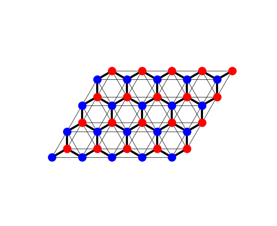
The Haldane model on a patch of \(5\times4\) cells (finite_system()), bond widths proportional to the amplitudes: the honeycomb lattice’s two sublattices (‘a’ and ‘b’, in two colours), the nearest-neighbour hopping (thick) and the complex second-neighbour hoppings \(\pm 0.2i\) (thin).

fig_lat = Plot(finite_system(hal, (5, 4))).lattice(plt_hop=True, ms=12, figsize=(5.5, 4.5))

Curvature and metric over the Brillouin zone

n = 30
fracs = (np.arange(n) + 0.5) / n
rec = hal.rec_vec_k
dA = abs(np.linalg.det(rec)) / n**2
omega = np.zeros((n, n))
trace_g = np.zeros((n, n))
for a, f1 in enumerate(fracs):
    for b, f2 in enumerate(fracs):
        q = hal.quantum_geometric_tensor(0, f1*rec[0] + f2*rec[1])
        omega[a, b] = -2 * q[0, 1].imag
        trace_g[a, b] = np.trace(q.real)
        assert np.sqrt(np.linalg.det(q.real)) >= abs(omega[a, b]) / 2 - 1e-8
chern = omega.sum() * dA / (2*np.pi)
print('Chern number from the curvature: {:.4f}'.format(chern))
assert np.isclose(chern, hal.chern_number(0, 30), atol=1e-3)
# the trace bound, integrated: int Tr g >= 2 pi |C|
print('Integrated Tr g = {:.3f} >= 2 pi |C| = {:.3f}'.format(trace_g.sum() * dA, 2*np.pi*abs(chern)))
assert trace_g.sum() * dA >= 2*np.pi*abs(chern) - 1e-6

fig, axes = plt.subplots(1, 2, figsize=(9.5, 4))
for ax, data, title in [(axes[0], omega, r'Berry curvature $\Omega_{xy}$'),
                              (axes[1], trace_g, r'quantum metric $\mathrm{Tr}\,g$')]:
    im = ax.imshow(data.T, origin='lower', extent=[0, 1, 0, 1], cmap='RdBu' if data is omega else 'viridis')
    ax.set_title(title)
    ax.set_xlabel('$k_1$ (fractional)')
    ax.set_ylabel('$k_2$ (fractional)')
    fig.colorbar(im, ax=ax)
fig.set_layout_engine('tight')

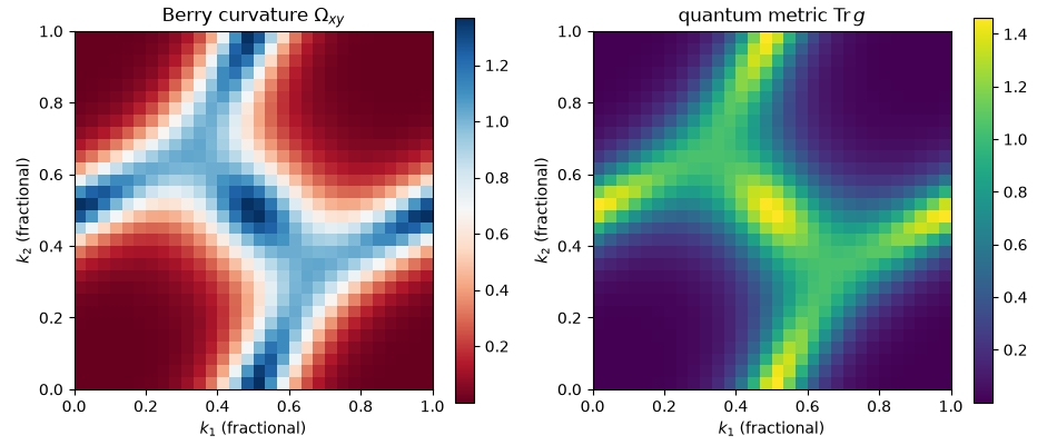
Chern number from the curvature: 1.0000
Integrated Tr g = 6.688 >= 2 pi |C| = 6.283