Exceptional Points in Momentum Space: Vorticity and Exceptional Rings

What becomes of a Dirac point when a Hermitian crystal is made non-Hermitian? It depends on the non-Hermitian term, and the answer is organized by a conserved quantity, the eigenvalue vorticity of Shen, Zhen and Fu (Phys. Rev. Lett. 120, 146402 (2018)),

\[\nu(\Gamma) = -\frac{1}{2\pi}\oint_\Gamma \nabla_{\mathbf{k}} \arg\left[E_+(\mathbf{k}) - E_-(\mathbf{k})\right]\cdot d\mathbf{k}\, .\]

A Dirac (diabolical) point has \(\nu = 0\): the gap \(E_+ - E_- = 2|f|\) is real and positive around it. A second-order exceptional point has \(\nu = \pm1/2\): \(E_+ - E_-\) is a square root that changes sign after one loop, so the two bands swap. As long as nothing crosses a loop \(\Gamma\), \(\nu(\Gamma)\) cannot change.

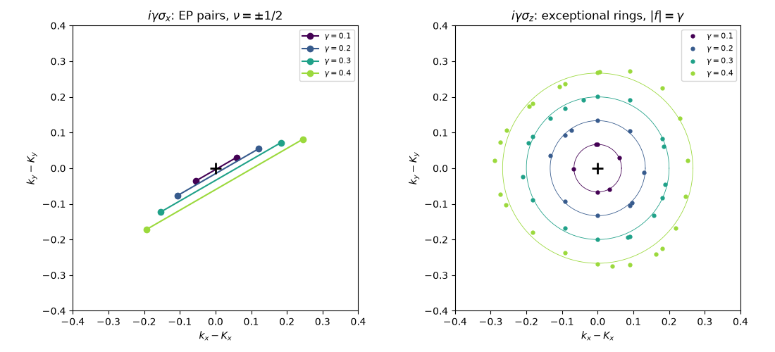
• A generic non-Hermitian term, here \(i\gamma\sigma_x\), splits the Dirac point into two EPs of vorticity \(+1/2\) and \(-1/2\), a distance \(\propto\gamma\) apart: the total around both stays 0.

• Balanced gain and loss on the two sublattices, \(i\gamma\sigma_z\), keeps \(\Delta = 4(|f|^2 - \gamma^2)\) real; the EPs are then not isolated but fill an exceptional ring \(|f(\mathbf{k})| = \gamma\) – the observation of Zhen et al. in a photonic crystal slab (Nature 525, 354 (2015)), where radiation losses play the part of \(\gamma\).

Near K, \(f \approx v_F(q_x \pm iq_y)\) up to a phase, with \(v_F = 3t/2\) (bond length 1), so the EP pair is split by \(2\gamma/v_F = 4\gamma/3\) and the ring has radius \(\gamma/v_F = 2\gamma/3\).

import numpy as np
import matplotlib.pyplot as plt

import tbkit.lattices as lattices
from tbkit.bridges import finite_system
from tbkit.kspace import KSpace
from tbkit.plot import Plot
import tbkit.exceptional as ex

NN = [{'i': 0, 'j': 1, 'R': (0, 0), 't': 1.}, {'i': 0, 'j': 1, 'R': (-1, 0), 't': 1.},
      {'i': 0, 'j': 1, 'R': (0, -1), 't': 1.}]
V_F = 1.5


def pair_model(gamma):
    '''Graphene + i gamma sigma_x.'''
    m = KSpace(lattices.honeycomb())
    m.set_hopping(NN)
    m.set_hopping([{'i': 0, 'j': 1, 'R': (0, 0), 't': 1j * gamma},
                   {'i': 1, 'j': 0, 'R': (0, 0), 't': 1j * gamma}], hermitian=False)
    return m


def ring_model(gamma):
    '''Graphene + balanced gain/loss, +i gamma on a, -i gamma on b.'''
    m = KSpace(lattices.honeycomb())
    m.set_hopping(NN)
    m.set_onsite({'a': 1j * gamma, 'b': -1j * gamma})
    return m


graphene = pair_model(0.)
b1, b2 = (np.array(b) for b in graphene.rec_vec_k)
K = (b1 - b2) / 3


def near_k(points, radius=0.6):
    '''Images of the points within radius of K, relative to K.'''
    shifts = [m * b1 + n * b2 for m in (-1, 0, 1) for n in (-1, 0, 1)]
    out = np.array([p + s - K for p in points for s in shifts]).reshape(-1, 2)
    return out[np.linalg.norm(out, axis=1) < radius]

The lattice

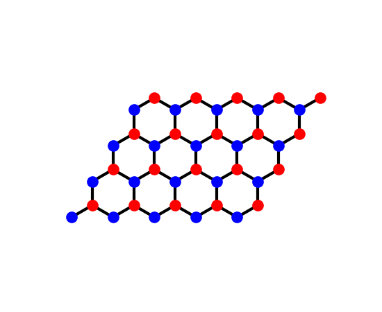
Graphene’s honeycomb lattice on a patch of \(5\times4\) cells (finite_system()): sublattices ‘a’ and ‘b’ in two colours, each bonded to its three nearest neighbours. The non-Hermitian terms below – \(i\gamma\) added to both directions of the intra-cell bond, or a gain and loss \(\pm i\gamma\) on the two sublattices – add no bond and are not drawn.

fig_lat = Plot(finite_system(graphene, (5, 4))).lattice(plt_hop=True, ms=12, figsize=(5.5, 4.5))

The Dirac point: vorticity 0

Around graphene’s K point the two bands do not swap, the discriminant \(\Delta = 4|f|^2\) is real and positive, and nothing is reported by the EP finder.

big_loop = ex.circle(K, 0.5)
nu_dp = ex.vorticity(graphene, big_loop)
print('graphene: vorticity {:.1e}, discriminant winding {:.1e}, EPs found: {}'
      .format(nu_dp, ex.discriminant_winding(graphene, big_loop),
              len(ex.find_exceptional_points(graphene, nk=30).k)))
assert abs(nu_dp) < 1e-10
assert len(ex.find_exceptional_points(graphene, nk=30).k) == 0

graphene: vorticity 2.9e-32, discriminant winding 3.6e-32, EPs found: 0

i gamma sigma_x: the Dirac point splits into a pair of EPs

For each \(\gamma\), the two EPs near K are located, their vorticities computed on small circles, and the total on the big circle around both. The individual vorticities are \(\pm1/2\), the total is the Dirac point’s 0, and the splitting follows \(4\gamma/3\) for small \(\gamma\) (the lattice corrections grow as \(\gamma^3\)).

gammas = [0.1, 0.2, 0.3, 0.4]
pairs = {}
for gamma in gammas:
    m = pair_model(gamma)
    pts = near_k(ex.find_exceptional_points(m, nk=40).k)
    assert len(pts) == 2
    pairs[gamma] = pts
    nus = [ex.vorticity(m, ex.circle(K + p, 0.02)) for p in pts]
    total = ex.vorticity(m, big_loop)
    split = np.linalg.norm(pts[0] - pts[1])
    print('gamma = {:.1f}: EP vorticities {:+.3f} {:+.3f}, total around both {:+.1e}, '
          'splitting {:.4f} (4 gamma / 3 = {:.4f})'.format(gamma, *nus, total, split, 4 * gamma / 3))
    assert np.allclose(sorted(nus), [-0.5, 0.5], atol=1e-10)
    assert abs(total) < 1e-10
    assert abs(ex.discriminant_winding(m, big_loop)) < 1e-10
    assert np.isclose(split, 2 * gamma / V_F, rtol=0.06)
assert np.isclose(np.linalg.norm(np.subtract(*pairs[0.1])), 4 * 0.1 / 3, rtol=0.005)

gamma = 0.1: EP vorticities +0.500 -0.500, total around both +1.8e-18, splitting 0.1329 (4 gamma / 3 = 0.1333)
gamma = 0.2: EP vorticities +0.500 -0.500, total around both +5.5e-19, splitting 0.2632 (4 gamma / 3 = 0.2667)
gamma = 0.3: EP vorticities +0.500 -0.500, total around both +1.3e-17, splitting 0.3886 (4 gamma / 3 = 0.4000)
gamma = 0.4: EP vorticities +0.500 -0.500, total around both +3.3e-17, splitting 0.5073 (4 gamma / 3 = 0.5333)

i gamma sigma_z: an exceptional ring

With balanced gain and loss the discriminant is real, so it vanishes on lines rather than at points. The finder samples them where they cross its mesh: every point lies on \(|f| = \gamma\), a ring of radius close to \(2\gamma/3\) around K. Crossing the ring changes the sign of \(\Delta\): outside, the two eigenvalues are real (\(\pm\sqrt{|f|^2-\gamma^2}\)); inside, they are imaginary, with equal real parts on a whole disk.

rings = {}
for gamma in gammas:
    m = ring_model(gamma)
    res = ex.find_exceptional_points(m, nk=40)
    pts = near_k(res.lines)
    rings[gamma] = pts
    moduli = np.array([abs(m.get_ham(K + p)[0, 1]) for p in pts])
    radius = np.linalg.norm(pts, axis=1)
    print('gamma = {:.1f}: {} ring points, |f| - gamma = {:.1e}, radius {:.4f} +- {:.4f} '
          '(2 gamma / 3 = {:.4f})'.format(gamma, len(pts), np.abs(moduli - gamma).max(),
                                          radius.mean(), radius.std(), 2 * gamma / 3))
    assert len(res.k) == 0 and len(pts) >= 6
    assert np.allclose(moduli, gamma, atol=1e-10)
    assert np.isclose(radius.mean(), gamma / V_F, rtol=0.05)
    inside = np.linalg.eigvals(m.get_ham(K))
    assert np.allclose(inside.real, 0., atol=1e-12)  # equal real parts inside the ring

gamma = 0.1: 6 ring points, |f| - gamma = 8.7e-16, radius 0.0670 +- 0.0006 (2 gamma / 3 = 0.0667)
gamma = 0.2: 10 ring points, |f| - gamma = 1.2e-15, radius 0.1336 +- 0.0033 (2 gamma / 3 = 0.1333)
gamma = 0.3: 18 ring points, |f| - gamma = 1.3e-15, radius 0.2013 +- 0.0070 (2 gamma / 3 = 0.2000)
gamma = 0.4: 24 ring points, |f| - gamma = 1.3e-15, radius 0.2717 +- 0.0130 (2 gamma / 3 = 0.2667)

EP pairs and rings around K

fig, axes = plt.subplots(1, 2, figsize=(11, 5))
colors = plt.cm.viridis(np.linspace(0., 0.85, len(gammas)))
for gamma, color in zip(gammas, colors):
    p = pairs[gamma]
    axes[0].plot(p[:, 0], p[:, 1], 'o-', color=color, label=r'$\gamma = {}$'.format(gamma))
    r = rings[gamma]
    axes[1].plot(r[:, 0], r[:, 1], '.', color=color, ms=7, label=r'$\gamma = {}$'.format(gamma))
    th = np.linspace(0., 2 * np.pi, 200)
    axes[1].plot(gamma / V_F * np.cos(th), gamma / V_F * np.sin(th), '-', color=color, lw=0.6)
for ax, title in ((axes[0], r'$i\gamma\sigma_x$: EP pairs, $\nu = \pm1/2$'),
                  (axes[1], r'$i\gamma\sigma_z$: exceptional rings, $|f| = \gamma$')):
    ax.plot(0., 0., 'k+', ms=12, mew=2)
    ax.set_aspect('equal')
    ax.set_xlim(-0.4, 0.4)
    ax.set_ylim(-0.4, 0.4)
    ax.set_xlabel(r'$k_x - K_x$')
    ax.set_ylabel(r'$k_y - K_y$')
    ax.set_title(title)
    ax.legend(fontsize=8)
fig.tight_layout()