The Landauer Formula: Quantized Conductance of a Point Contact

R. Landauer (1957), then M. Buttiker (1986), recast electrical conductance as a scattering problem: a phase-coherent conductor between two reservoirs has, at zero temperature and bias,

\[G = \frac{e^2}{h}\,T(E_F)\, ,\qquad T = \mathrm{Tr}\left[\Gamma_R\,G^r\,\Gamma_L\,G^a\right]\, ,\]

the (Caroli) transmission summed over the transverse modes of the leads. A perfect wire transmits every open mode fully, so its conductance counts them: it is quantized in units of \(e^2/h\) (per spin). In 1988 van Wees et al. and Wharam et al. saw exactly this in a quantum point contact, a constriction narrowed by a gate in a two-dimensional electron gas: the conductance fell in steps as the gate closed the modes one by one.

Transport attaches semi-infinite leads (strips cut from the square lattice with ribbon(), their surface Green’s functions from the Sancho-Rubio decimation) to a finite strip, and computes \(T(E)\). A smooth saddle-shaped potential – Buttiker’s model of a point contact – reproduces the steps.

import numpy as np
import matplotlib.pyplot as plt

import tbkit.lattices as lattices
from tbkit.kspace import ribbon
from tbkit.plot import Plot
from tbkit.system import System
from tbkit.transport import Transport, lead_from_kspace


t = -1.
width, length = 24, 40
square = [{'i': 0, 'j': 0, 'R': (1, 0), 't': t}, {'i': 0, 'j': 0, 'R': (0, 1), 't': t}]

lat = lattices.square()
lat.get_lattice(length, width)
x = lat.coor['x'] - (length - 1) / 2
y = lat.coor['y'] - (width - 1) / 2
left = list(np.flatnonzero(np.isclose(lat.coor['x'], 0.)))
right = list(np.flatnonzero(np.isclose(lat.coor['x'], length - 1.)))

# the leads: the same strip, continued to -x and to +x
strip = ribbon(lattices.square(), square, width=width, direction=1)
h_left, v_left = lead_from_kspace(strip, -1)
h_right, v_right = lead_from_kspace(strip, 1)


def device(potential):
    sys = System(lat)
    sys.set_hopping([{'n': 1, 't': t}])
    sys.set_onsite({'a': 0.})
    sys.onsite[:] = potential
    sys.get_ham()
    tr = Transport(sys.ham)
    # device edge site at height y couples to the lead orbital at the same y
    tr.add_lead(h_left, v_left, t * np.eye(width), left)
    tr.add_lead(h_right, v_right, t * np.eye(width), right)
    return tr

The device

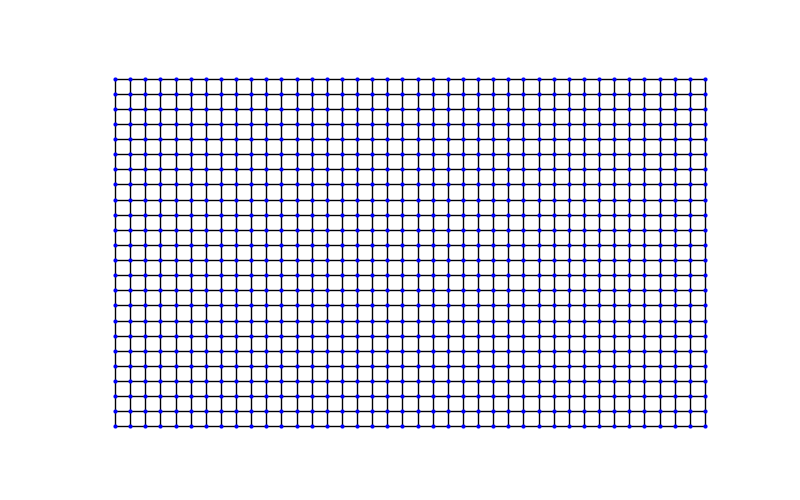
A \(40\times24\) strip of the square lattice with its nearest-neighbour bonds, between two semi-infinite leads that continue the strip to the left and right. The gate potential below acts on its onsite energies.

vis = System(lat)
vis.set_hopping([{'n': 1, 't': t}])
fig_lat = Plot(vis).lattice(plt_hop=True, ms=3, c=1., figsize=(8, 5))

A clean strip counts its open modes

The transverse modes of the strip have energies \(2t\cos(n\pi/(W+1))\); at energy \(E\), mode \(n\) is open if \(|E - 2t\cos(n\pi/(W+1))| < 2|t|\).

energies = np.linspace(-3.9, 0., 40)
clean = device(np.zeros(lat.sites)).transmission(energies)
modes = [sum(abs(e - 2*t*np.cos(n*np.pi/(width + 1))) < 2*abs(t) for n in range(1, width + 1))
             for e in energies]
assert np.allclose(clean, modes, atol=1e-6)
print('Clean strip: T(E) equals the number of open modes at every energy.')

Clean strip: T(E) equals the number of open modes at every energy.

A point contact: conductance steps as the gate closes it

The saddle \(V(x, y) = (V_g + \omega_y y^2)\cos^2(\pi x/L)\) pinches the strip in the middle and vanishes smoothly at the leads.

envelope = np.cos(np.pi * x / (length - 1)) ** 2
gates = np.linspace(1.0, -0.4, 57)
e_fermi = -3.
conductance = np.array([device((vg + 0.02 * y**2) * envelope).transmission([e_fermi])[0]
                                     for vg in gates])
for n in range(1, 5):
    closest = np.min(np.abs(conductance - n))
    print('Plateau at G = {} e^2/h: reached within {:.3f}'.format(n, closest))
    assert closest < 0.01
assert conductance[0] < 0.05 and np.all(np.diff(conductance) > -0.05)

fig, ax = plt.subplots(figsize=(6, 4))
ax.plot(gates, conductance, 'o-b', ms=3)
ax.set_xlabel('gate potential $V_g$')
ax.set_ylabel('$G$ ($e^2/h$)')
ax.set_yticks(range(0, 7))
ax.grid(axis='y', alpha=0.4)
ax.invert_xaxis()
ax.set_title('Quantum point contact: conductance quantization')
fig.set_layout_engine('tight')

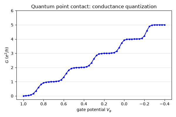
Plateau at G = 1 e^2/h: reached within 0.000
Plateau at G = 2 e^2/h: reached within 0.000
Plateau at G = 3 e^2/h: reached within 0.001
Plateau at G = 4 e^2/h: reached within 0.000