The Anomalous Hall Effect: from the Anomalous Velocity to the Berry Phase

In 1954 Karplus and Luttinger found that the electrons of a ferromagnet acquire an anomalous velocity transverse to an applied electric field, a Hall current with no magnetic field. Half a century later it was recognized as a Berry-phase effect (Jungwirth, Niu and MacDonald 2002; Haldane 2004): a band’s velocity picks up \(-\dot{\mathbf{k}}\times \boldsymbol\Omega_n(\mathbf{k})\), and the intrinsic Hall conductivity is the Berry curvature summed over the occupied states,

\[\sigma_{xy}(E_F) = \frac{e^2}{h}\,\frac{1}{2\pi}\int_{BZ} d^2k\, \sum_n f(E_n)\,\Omega_n(\mathbf{k})\, .\]

In a gap, every band is either full or empty, and the integral is the Chern number: the quantum anomalous Hall effect. Inside a band, it is whatever fraction of the curvature lies below the Fermi level – not quantized, and no longer zero even in a topologically trivial phase.

hall_conductivity() evaluates the Kubo formula behind it at any Fermi level, for the Haldane model below (the sign is that of chern_number(), see its docstring).

import numpy as np
import matplotlib.pyplot as plt

import tbkit.lattices as lattices
from tbkit.bridges import finite_system
from tbkit.kspace import KSpace
from tbkit.plot import Plot


def haldane(M, t2=0.2):
    '''Haldane model: nearest-neighbour t = 1, i t2 on the second neighbours, mass +-M.'''
    hal = KSpace(lattices.honeycomb())
    hal.set_hopping([{'i': 0, 'j': 1, 'R': R, 't': 1.} for R in [(0, 0), (-1, 0), (0, -1)]])
    for R in [(0, 1), (-1, 0), (1, -1)]:  # a2, -a1, a1 - a2: 120 degrees apart
        hal.set_hopping([{'i': 0, 'j': 0, 'R': R, 't': 1j*t2}, {'i': 1, 'j': 1, 'R': R, 't': -1j*t2}])
    hal.set_onsite({'a': M, 'b': -M})
    return hal

The lattice

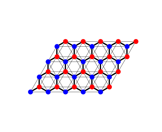
The Haldane model on a patch of \(5\times4\) cells (finite_system()), each bond drawn with a width proportional to its amplitude: the honeycomb lattice’s two sublattices (‘a’ and ‘b’, in two colours), the nearest-neighbour hopping \(t\) (thick) and the complex second-neighbour hoppings \(\pm it_2\) within each sublattice (thin), which break time-reversal symmetry.

fig_lat = Plot(finite_system(haldane(0.3), (5, 4))).lattice(plt_hop=True, ms=12, figsize=(5.5, 4.5))

The Hall conductivity across the spectrum

One diagonalization of a 150 x 150 mesh gives every Fermi level at once. The topological phase (\(M = 0.3\), below Haldane’s \(M_c = 3\sqrt3\,t_2 \approx 1.04\)) and the trivial one (\(M = 1.5\)):

e_f = np.linspace(-3.6, 3.6, 721)
phases = {'topological, M = 0.3': haldane(0.3), 'trivial, M = 1.5': haldane(1.5)}
sigma = {name: hal.hall_conductivity(e_f, nk=150) for name, hal in phases.items()}

for name, hal in phases.items():
    en = hal.mesh_bands(150)
    gap = (en[:, 0].max(), en[:, 1].min())
    chern = hal.chern_number([0], 60)
    in_gap = (e_f > gap[0] + 0.02) & (e_f < gap[1] - 0.02)
    plateau = sigma[name][in_gap]
    print('{}: gap ({:.3f}, {:.3f}), C = {:.4f}, sigma_xy in the gap from {:.6f} to {:.6f} e^2/h'.format(
        name, *gap, chern, plateau.min(), plateau.max()))
    # the plateau is the Chern number
    assert np.allclose(plateau, chern, atol=1e-6)
    # an empty and a full model carry no Hall current
    assert sigma[name][0] == 0. and abs(sigma[name][-1]) < 1e-10

# Inside the bands the value is not quantized: at E_F = -1.2, in the
# upper part of the lower band, it is far from any integer in both phases
# -- nonzero even in the trivial phase.
e_band = -1.2
mid = np.argmin(np.abs(e_f - e_band))
for name in phases:
    print('{}: sigma_xy(E_F = {:.2f}) = {:.4f} e^2/h'.format(name, e_f[mid], sigma[name][mid]))
    assert 0.1 < sigma[name][mid] < 0.9

fig, ax = plt.subplots(figsize=(7, 4.5))
for (name, s), color in zip(sigma.items(), ('C0', 'C3')):
    ax.plot(e_f, s, color=color, label=name)
ax.axhline(1., color='k', lw=0.5, ls=':')
ax.axhline(0., color='k', lw=0.5)
ax.set_xlabel('$E_F$')
ax.set_ylabel(r'$\sigma_{xy}$ ($e^2/h$)')
ax.set_title('Haldane model: anomalous Hall conductivity')
ax.legend()

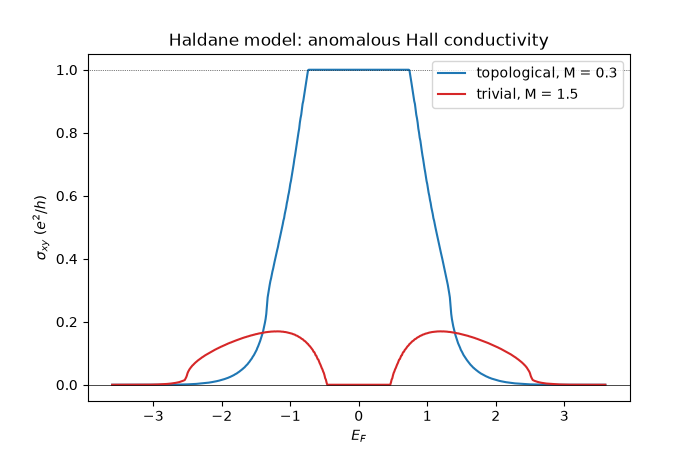
topological, M = 0.3: gap (-0.739, 0.739), C = 1.0000, sigma_xy in the gap from 1.000000 to 1.000000 e^2/h
trivial, M = 1.5: gap (-0.461, 0.461), C = -0.0000, sigma_xy in the gap from -0.000000 to -0.000000 e^2/h
topological, M = 0.3: sigma_xy(E_F = -1.20) = 0.4184 e^2/h
trivial, M = 1.5: sigma_xy(E_F = -1.20) = 0.1695 e^2/h

<matplotlib.legend.Legend object at 0x10f311e80>

Where the curvature sits

Filling the lower band adds the curvature of its states, from the bottom up. In the topological phase the curvature has one sign over the whole band, peaked near K and K’ at its top, so \(\sigma_{xy}\) rises monotonically to \(C = 1\). In the trivial phase the curvature at K and at K’ have opposite signs (the mass term dominates the Haldane term at one valley and not at the other), so \(\sigma_{xy}\) rises and then falls back to exactly 0 as the band fills: a Hall current carried by a metal whose filled bands are topologically trivial.

lower = e_f < -0.74
topo, triv = sigma['topological, M = 0.3'][lower], sigma['trivial, M = 1.5'][lower]
assert np.all(np.diff(topo) >= -1e-9)
peak = np.argmax(triv)
print('trivial phase: sigma_xy peaks at {:.3f} e^2/h for E_F = {:.2f}'.format(triv[peak], e_f[lower][peak]))
assert triv[peak] > 0.15 and np.all(np.diff(triv[peak:][e_f[lower][peak:] > -0.46]) <= 1e-9)

trivial phase: sigma_xy peaks at 0.170 e^2/h for E_F = -1.20

Temperature and convergence

A finite temperature smooths the band edges (the Fermi-Dirac tails empty the top of the lower band), and speeds up the convergence in the mesh: at \(T = 0.05\), a 60 x 60 mesh already agrees with 240 x 240 to \(10^{-4}\) in the bands.

hal = phases['topological, M = 0.3']
e_band = np.array([-2.2, -1.4, 1.2])
coarse = hal.hall_conductivity(e_band, temperature=0.05, nk=60)
fine = hal.hall_conductivity(e_band, temperature=0.05, nk=240)
print('T = 0.05, nk = 60 vs 240: max difference {:.2e}'.format(np.max(np.abs(coarse - fine))))
assert np.max(np.abs(coarse - fine)) < 1e-4

warm = hal.hall_conductivity(e_f, temperature=0.1, nk=150)
fig2, ax2 = plt.subplots(figsize=(7, 4.5))
ax2.plot(e_f, sigma['topological, M = 0.3'], label='$T = 0$')
ax2.plot(e_f, warm, label='$T = 0.1$')
ax2.set_xlabel('$E_F$')
ax2.set_ylabel(r'$\sigma_{xy}$ ($e^2/h$)')
ax2.set_title('Topological phase: the plateau at $C = 1$, smoothed by temperature')
ax2.legend()

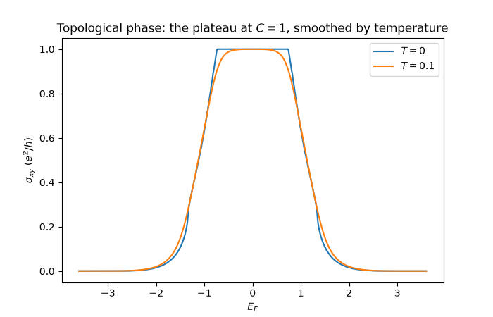
T = 0.05, nk = 60 vs 240: max difference 1.37e-07

<matplotlib.legend.Legend object at 0x10f536e40>