The Bott Index: the Chern Number of a Disordered Torus

The Chern number is an integral over the Brillouin zone, and disorder removes the Brillouin zone. T. Loring and M. Hastings (2010) found an invariant of a finite sample that needs none. Put the sample on a torus, where the coordinates \(X_1, X_2\) (in units of the torus sides) are only defined modulo 1, but their exponentials \(e^{2\pi iX_{1,2}}\) are well defined. Project them onto the occupied states, \(\tilde U = Pe^{2\pi iX_1}P\) and \(\tilde V = Pe^{2\pi iX_2}P\). In a gapped or localized phase they almost commute, and the winding of their commutator,

\[B = \frac{1}{2\pi}\,\mathrm{Im}\,\mathrm{Tr}\log\left(\tilde V\tilde U\tilde V^\dagger\tilde U^\dagger\right)\, ,\]

is an integer: the Bott index. It equals the Chern number of a clean crystal. Unlike the local Chern marker (get_local_chern_marker(), which needs open edges and a bulk average), it is a single integer for the whole sample, and it applies to any set of positions: amorphous solids, quasicrystals, disordered lattices.

bott_index() computes it from a Hamiltonian on a torus (finite_ham() with periodic=True) and the orbital positions (flake_positions()), here for the Haldane model with Anderson disorder.

import numpy as np
import matplotlib.pyplot as plt

import tbkit.lattices as lattices
from tbkit.bridges import finite_system
from tbkit.higher_order import flake_positions
from tbkit.kspace import KSpace
from tbkit.plot import Plot
from tbkit.topology import bott_index


def haldane(t2=0.2, M=0.):
    hal = KSpace(lattices.honeycomb())
    hal.set_hopping([{'i': 0, 'j': 1, 'R': R, 't': 1.} for R in [(0, 0), (-1, 0), (0, -1)]])
    for R in [(0, 1), (-1, 0), (1, -1)]:
        hal.set_hopping([{'i': 0, 'j': 0, 'R': R, 't': 1j*t2}, {'i': 1, 'j': 1, 'R': R, 't': -1j*t2}])
    hal.set_onsite({'a': M, 'b': -M})
    return hal


n = 14  # a 14 x 14-cell torus, 392 sites
positions = flake_positions(haldane(), (n, n))
cell = [n * np.array(a) for a in haldane().lat.prim_vec]

The lattice

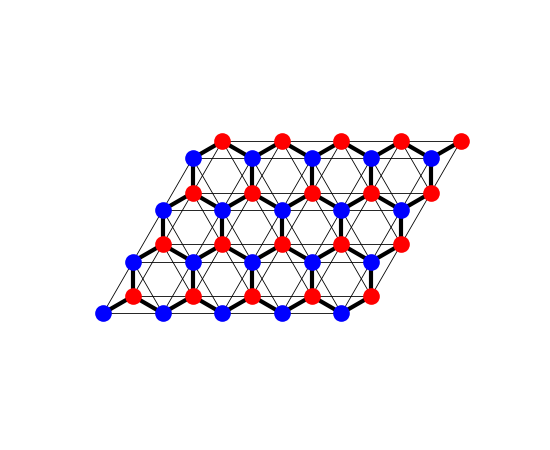
The Haldane model on a patch of \(5\times4\) cells (finite_system()), each bond drawn with a width proportional to its amplitude: the honeycomb lattice’s two sublattices (‘a’ and ‘b’, in two colours), the nearest-neighbour hopping \(t\) (thick) and the complex second-neighbour hoppings \(\pm it_2\) within each sublattice (thin), which break time-reversal symmetry. The torus below is \(14\times14\) cells.

fig_lat = Plot(finite_system(haldane(), (5, 4))).lattice(plt_hop=True, ms=12, figsize=(5.5, 4.5))

Clean tori: the Bott index is the Chern number

for t2, M in ((0.2, 0.), (0.2, 0.5), (0.2, 1.5), (-0.2, 0.)):
    hal = haldane(t2, M)
    bott = bott_index(hal.finite_ham((n, n), periodic=True), positions, cell)
    chern = hal.chern_number(0, 30)
    print('t2 = {:+.1f}, M = {:.1f}: Bott index {:+.3f}, Chern number {:+.3f}'.format(t2, M, bott, chern))
    assert np.isclose(bott, chern, atol=1e-6)

t2 = +0.2, M = 0.0: Bott index +1.000, Chern number +1.000
t2 = +0.2, M = 0.5: Bott index +1.000, Chern number +1.000
t2 = +0.2, M = 1.5: Bott index +0.000, Chern number +0.000
t2 = -0.2, M = 0.0: Bott index -1.000, Chern number -1.000

Disorder: quantized until the mobility gap closes

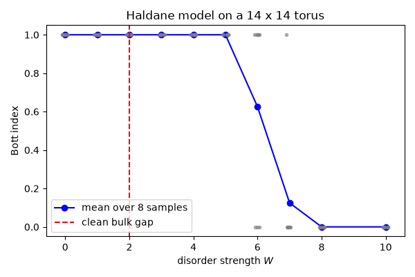
Random onsite energies in \([-W/2, W/2]\). The clean bulk gap is 2.0, yet the Bott index stays exactly 1 for every sample up to \(W = 5\): the states disorder pushes into the gap are localized and do not change the topology. Only when the extended states of the two bands meet (the topological Anderson transition, near \(W \approx 6\) here) does it drop to 0, sample by sample.

hal = haldane()
ham = hal.finite_ham((n, n), periodic=True)
bands = hal.mesh_bands(60)
clean_gap = np.min(bands[:, 1] - bands[:, 0])
print('clean bulk gap: {:.2f}'.format(clean_gap))
assert np.isclose(clean_gap, 2., atol=0.01)
rng = np.random.default_rng(0)
disorder = np.array([0., 1., 2., 3., 4., 5., 6., 7., 8., 10.])
n_samples = 8
botts = np.array([[bott_index(ham + np.diag(rng.uniform(-w / 2, w / 2, len(ham))), positions, cell)
                          for _ in range(n_samples)] for w in disorder])
assert np.allclose(botts, np.round(botts), atol=1e-6)  # an integer for every sample
botts = np.round(botts).astype(int)
for w, b in zip(disorder, botts):
    print('W = {:4.1f}: Bott indices {}'.format(w, b.tolist()))
assert np.all(botts[disorder <= 5.] == 1) and np.all(botts[disorder >= 8.] == 0)

fig, ax = plt.subplots(figsize=(6, 4))
ax.plot(disorder, botts.mean(axis=1), 'o-b', label='mean over {} samples'.format(n_samples))
for w, b in zip(disorder, botts):
    ax.plot(np.full(n_samples, w) + rng.uniform(-0.1, 0.1, n_samples), b, '.', color='gray', alpha=0.6)
ax.axvline(clean_gap, color='r', ls='--', label='clean bulk gap')
ax.set_xlabel('disorder strength $W$')
ax.set_ylabel('Bott index')
ax.set_title('Haldane model on a {0} x {0} torus'.format(n))
ax.legend()
fig.set_layout_engine('tight')

clean bulk gap: 2.00
W =  0.0: Bott indices [1, 1, 1, 1, 1, 1, 1, 1]
W =  1.0: Bott indices [1, 1, 1, 1, 1, 1, 1, 1]
W =  2.0: Bott indices [1, 1, 1, 1, 1, 1, 1, 1]
W =  3.0: Bott indices [1, 1, 1, 1, 1, 1, 1, 1]
W =  4.0: Bott indices [1, 1, 1, 1, 1, 1, 1, 1]
W =  5.0: Bott indices [1, 1, 1, 1, 1, 1, 1, 1]
W =  6.0: Bott indices [0, 1, 0, 1, 1, 1, 0, 1]
W =  7.0: Bott indices [0, 0, 1, 0, 0, 0, 0, 0]
W =  8.0: Bott indices [0, 0, 0, 0, 0, 0, 0, 0]
W = 10.0: Bott indices [0, 0, 0, 0, 0, 0, 0, 0]