The Scaling Theory of Localization: the 3D Anderson Transition

Abrahams, Anderson, Licciardello and Ramakrishnan (1979) argued that the conductance of a disordered sample flows, as its size \(L\) grows, according to a single scaling function of the conductance itself. The consequence: in one and two dimensions every state is localized by any disorder, but in three dimensions a genuine metal-insulator transition survives, at a critical disorder – \(W_c \approx 16.5\,t\) for the Anderson model on the cubic lattice, with onsite energies uniform in \([-W/2, W/2]\).

The transition shows in the statistics of the energy levels. Extended states repel each other, and their spacings follow random-matrix (GOE) statistics; localized states are independent, with Poisson statistics. The mean ratio of consecutive spacings \(r_n = \min(s_n, s_{n+1})/\max(s_n, s_{n+1})\) tells them apart – \(\langle r\rangle \approx 0.5307\) (GOE), \(0.3863\) (Poisson) – and, as \(L\) grows, flows towards the first value in the metal and towards the second in the insulator: the curves for two sizes cross at the transition.

import numpy as np
import matplotlib.pyplot as plt
from mpl_toolkits.mplot3d.art3d import Line3DCollection

from tbkit.lattice import Lattice
from tbkit.system import System

R_GOE, R_POISSON = 0.5307, 0.3863
cubic = [(1., 0., 0.), (0., 1., 0.), (0., 0., 1.)]


def anderson(L):
    lat = Lattice(unit_cell=[{'tag': 'a', 'r0': (0., 0., 0.)}], prim_vec=cubic)
    lat.get_lattice(L, L, L)
    sys = System(lat)
    sys.set_hopping([{'n': 1, 't': 1.}])
    return sys


def mean_ratio(sys, W, samples, seed=0):
    '''<r> over the central 40% of the spectrum, averaged over disorder samples.'''
    np.random.seed(seed)
    ratios = []
    for _ in range(samples):
        sys.set_onsite({'a': 0.})
        sys.set_onsite_dis(W / 2)  # uniform in [-W/2, W/2]
        sys.get_ham()
        sys.get_eig()
        en = np.sort(sys.en)
        mid = en[int(0.3 * len(en)):int(0.7 * len(en))]
        s = np.diff(mid)
        ratios.append(np.mean(np.minimum(s[1:], s[:-1]) / np.maximum(s[1:], s[:-1])))
    return np.mean(ratios), np.std(ratios) / np.sqrt(samples)

The lattice

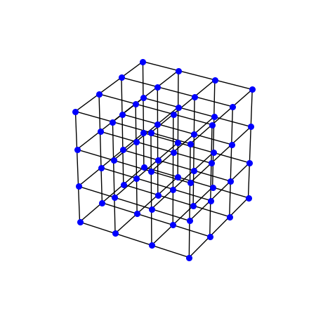
The simple cubic lattice, one site per cell and six nearest neighbours, here \(4\times4\times4\) sites of it. Each site gets a random onsite energy in \([-W/2, W/2]\).

lat_vis = Lattice(unit_cell=[{'tag': 'a', 'r0': (0., 0., 0.)}], prim_vec=cubic)
lat_vis.get_lattice(4, 4, 4)
vis = System(lat_vis)
vis.set_hopping([{'n': 1, 't': 1.}])
pos = np.column_stack([lat_vis.coor[f] for f in 'xyz'])
bonds = np.stack([pos[vis.hop['i'].astype(int)], pos[vis.hop['j'].astype(int)]], axis=1)
fig_lat = plt.figure(figsize=(4.5, 4.5))
ax_lat = fig_lat.add_subplot(projection='3d')
ax_lat.add_collection3d(Line3DCollection(bonds, colors='k', linewidths=1))
ax_lat.scatter(*pos.T, s=30, c='b', depthshade=False)
ax_lat.set_aspect('equal')
ax_lat.set_axis_off()

Level statistics across the transition

disorders = [4., 8., 12., 16.5, 20., 25., 35.]
sizes = {6: 60, 10: 20}  # L: disorder samples
curves = {L: np.array([mean_ratio(anderson(L), W, n) for W in disorders]) for L, n in sizes.items()}
for L, curve in curves.items():
    print('L = {:2d}: <r> ='.format(L), np.round(curve[:, 0], 3))

# weak disorder: extended states, random-matrix statistics; strong
# disorder: localized, close to Poisson
assert abs(curves[10][0, 0] - R_GOE) < 0.015 and abs(curves[6][0, 0] - R_GOE) < 0.015
assert curves[6][-1, 0] < 0.415 and curves[10][-1, 0] < 0.415


def grows(W):
    """Does <r> grow from L = 6 to L = 10 at disorder W (by more than 2 sigma)?"""
    (r6, e6), (r10, e10) = curves[6][disorders.index(W)], curves[10][disorders.index(W)]
    return (r10 - r6) / np.hypot(e6, e10)


# the scaling signature: below W_c the larger sample is more metallic,
# above it more insulating -- the curves cross in between
assert grows(12.) > 2 and grows(20.) < -2
print('<r> grows with L at W = 12 ({:+.1f} sigma), shrinks at W = 20 ({:+.1f} sigma): '
          'the curves cross between them, around W_c = 16.5.'.format(grows(12.), grows(20.)))

fig, ax = plt.subplots(figsize=(6.2, 4))
for L, curve in curves.items():
    ax.errorbar(disorders, curve[:, 0], yerr=curve[:, 1], fmt='o-', ms=4, label='$L = {}$'.format(L))
ax.axhline(R_GOE, color='k', ls=':', lw=1)
ax.axhline(R_POISSON, color='k', ls=':', lw=1)
ax.axvline(16.5, color='0.5', ls='--', lw=1)
ax.text(4.5, R_GOE + 0.005, 'GOE (metal)')
ax.text(4.5, R_POISSON + 0.005, 'Poisson (insulator)')
ax.set_xlabel('disorder $W/t$')
ax.set_ylabel(r'$\langle r\rangle$')
ax.legend()
ax.set_title('3D Anderson transition ($W_c \\approx 16.5\\,t$)')
fig.set_layout_engine('tight')

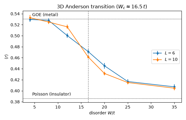
L =  6: <r> = [0.53  0.528 0.5   0.471 0.445 0.417 0.407]
L = 10: <r> = [0.533 0.525 0.516 0.461 0.431 0.415 0.405]
<r> grows with L at W = 12 (+2.9 sigma), shrinks at W = 20 (-2.3 sigma): the curves cross between them, around W_c = 16.5.