TKNN: The Quantized Hall Conductance of the Hofstadter Bands

Thouless, Kohmoto, Nightingale and den Nijs (1982) computed the Hall conductance of electrons on a lattice in a magnetic field, and found it to be a topological integer – the first Chern number of the occupied bands. For a flux \(\alpha = p/q\) per plaquette, the square lattice’s band splits into \(q\) Hofstadter subbands, and the Hall conductance with \(r\) bands filled, \(\sigma_{xy} = t_r\,e^2/h\), solves the Diophantine equation

\[r = q\,s_r + p\,t_r\, ,\qquad |t_r| \le q/2\, ,\]

so that each band carries \(C_r = t_r - t_{r-1}\).

magnetic_supercell() builds the magnetic unit cell of \(q\) plaquettes, with the Peierls phases of the field, and chern_number() integrates each subband’s Berry curvature: the numbers come out as TKNN’s integers.

import numpy as np
import matplotlib.pyplot as plt

import tbkit.lattices as lattices
from tbkit.bridges import finite_system
from tbkit.kspace import magnetic_supercell
from tbkit.plot import Plot


square = [{'i': 0, 'j': 0, 'R': (1, 0), 't': 1.}, {'i': 0, 'j': 0, 'R': (0, 1), 't': 1.}]


def tknn(p, q, r):
    '''t_r from the Diophantine equation r = q s + p t, |t| <= q/2.'''
    return next(t for t in range(-q, q + 1) if (r - p*t) % q == 0 and abs(t) <= q/2)

The lattice

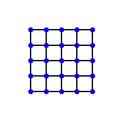
The square lattice, one site per cell and a nearest-neighbour hopping, here as five of its magnetic cells at flux \(1/5\) (magnetic_supercell(), then finite_system()): five sites along \(\mathbf{a}_1\) per magnetic cell. The Peierls phases change the hoppings’ phases, not their amplitudes, so every bond is drawn alike.

fig_lat = Plot(finite_system(magnetic_supercell(lattices.square(), square, 1, 5), (1, 5))).lattice(plt_hop=True, ms=12, figsize=(4, 4))

Chern numbers of the subbands, against the Diophantine equation

for p, q in [(1, 3), (1, 5), (2, 5), (3, 7)]:
    mag = magnetic_supercell(lattices.square(), square, p, q)
    chern = np.array([mag.chern_number([n], nk=20) for n in range(q)])
    expected = [tknn(p, q, r + 1) - tknn(p, q, r) for r in range(q)]
    print('alpha = {}/{}: C = {}  (TKNN: {})'.format(p, q, np.round(chern).astype(int), expected))
    assert np.allclose(chern, expected, atol=1e-6)
    assert np.isclose(chern.sum(), 0., atol=1e-6)

alpha = 1/3: C = [ 1 -2  1]  (TKNN: [1, -2, 1])
alpha = 1/5: C = [ 1  1 -4  1  1]  (TKNN: [1, 1, -4, 1, 1])
alpha = 2/5: C = [-2  3 -2  3 -2]  (TKNN: [-2, 3, -2, 3, -2])
alpha = 3/7: C = [-2  5 -2 -2 -2  5 -2]  (TKNN: [-2, 5, -2, -2, -2, 5, -2])

The Hall conductance in each gap

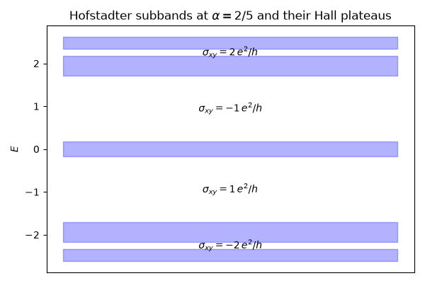
\(\sigma_{xy}\) with the lowest \(r\) bands filled is the sum of their Chern numbers, \(t_r\): for \(\alpha = 2/5\), the plateaus \(-2, 1, -1, 2\).

p, q = 2, 5
mag = magnetic_supercell(lattices.square(), square, p, q)
bands = mag.mesh_bands(20)
sigma = np.cumsum([mag.chern_number([n], nk=20) for n in range(q)])[:-1]
assert np.allclose(sigma, [tknn(p, q, r) for r in range(1, q)], atol=1e-6)
assert np.allclose(sigma, [-2, 1, -1, 2], atol=1e-6)
fig, ax = plt.subplots(figsize=(6, 4))
for n in range(q):
    ax.fill_between([0, 1], bands[:, n].min(), bands[:, n].max(), color='b', alpha=0.3)
for r in range(1, q):
    e_gap = (bands[:, r - 1].max() + bands[:, r].min()) / 2
    ax.text(0.5, e_gap, r'$\sigma_{xy} = %d\,e^2/h$' % round(sigma[r - 1]), ha='center', va='center')
ax.set_xticks([])
ax.set_ylabel('$E$')
ax.set_title(r'Hofstadter subbands at $\alpha = 2/5$ and their Hall plateaus')
fig.set_layout_engine('tight')