Buttiker’s Edge Channels: the Quantized Resistances of a Hall Bar

Buttiker (1986) wrote the currents of a phase-coherent conductor with many leads as \(I_p = \frac{e^2}{h}\sum_q G_{pq}V_q\), from the transmissions between leads, and treated voltage probes as leads that draw no net current. In 1988 he applied it to the quantum Hall effect: in a strong field the current flows in \(\nu\) chiral edge channels, one per filled Landau level, which carry electrons from each contact to the next one downstream without backscattering. The Landauer-Buttiker equations then give, for any sample shape and any probes,

\[R_{xy} = \frac{h}{\nu e^2}\, ,\qquad R_{xx} = 0\, ,\]

the exact quantization of von Klitzing’s plateaus (1980) and the vanishing longitudinal resistance between them.

A square-lattice Hall bar in a perpendicular field (flux 0.05 flux quanta per plaquette, in the Landau gauge through set_peierls_phase()) gets six leads: the current source (0) and drain (5) continue the bar, four voltage probes sit on its edges. conductance_matrix() and four_terminal_resistance() solve the Landauer-Buttiker equations; local_currents() maps the current.

import numpy as np
import matplotlib.pyplot as plt

import tbkit.lattices as lattices
from tbkit.plot import Plot
from tbkit.system import System
from tbkit.transport import Transport

t, flux, length, width, probe = -1., 0.05, 44, 16, 6

lat = lattices.square()
lat.get_lattice(length, width)
x, y = lat.coor['x'], lat.coor['y']
sys = System(lat)
sys.set_hopping([{'n': 1, 't': t}])
sys.set_onsite({'a': 0.})
# Landau gauge A = (-B y, 0): only the bonds along x pick up a phase
sys.set_peierls_phase(lambda xi, yi, xj, yj: -2 * np.pi * flux * (xj - xi) * (yi + yj) / 2)
sys.get_ham()
ham = sys.ham.toarray()

bar = Transport(ham)
cols = [sorted(np.flatnonzero(np.isclose(x, c)), key=lambda i: y[i]) for c in (0, 1, length - 2, length - 1)]
cols = [[int(i) for i in c] for c in cols]
# lead 0 (source): the bar continued to -x, same gauge
v = ham[np.ix_(cols[1], cols[0])]
bar.add_lead(ham[np.ix_(cols[0], cols[0])], v, v, cols[0])
# leads 1, 2 (top edge) and 3, 4 (bottom edge): field-free strips along y
h_probe = t * (np.eye(probe, k=1) + np.eye(probe, k=-1))
for edge in (width - 1, 0):
    for x0 in (length // 4 - probe // 2, 3 * length // 4 - probe // 2):
        sites = [int(np.flatnonzero(np.isclose(x, x0 + k) & np.isclose(y, edge))[0]) for k in range(probe)]
        bar.add_lead(h_probe, t * np.eye(probe), t * np.eye(probe), sites)
# lead 5 (drain): the bar continued to +x
v = ham[np.ix_(cols[2], cols[3])]
bar.add_lead(ham[np.ix_(cols[3], cols[3])], v, v, cols[3])

The Hall bar

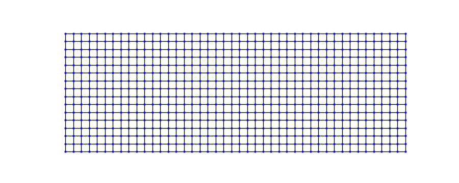
A \(44\times16\) strip of the square lattice with its nearest-neighbour bonds (their Peierls phases are not drawn). The source and drain leads continue it to the left and right; the four probes are strips of six sites attached along the top and bottom edges.

fig_lat = Plot(sys).lattice(plt_hop=True, ms=3, c=1., figsize=(9, 3.6))

Quantized plateaus

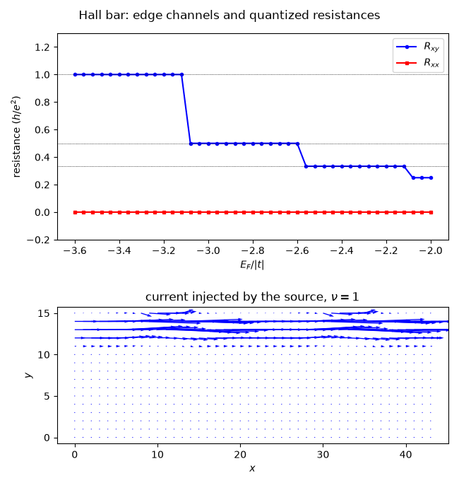
The Landau levels sit near \(-4|t| + 4\pi\phi|t|(n + \frac12)\), \(\phi\) the flux per plaquette; between them \(\nu\) edge channels carry the current.

e_fermi = np.linspace(-3.6, -2.0, 41)
r_xy, r_xx = [], []
for e in e_fermi:
    r_xy.append(bar.four_terminal_resistance(e, current=(0, 5), voltage=(1, 3)))
    r_xx.append(bar.four_terminal_resistance(e, current=(0, 5), voltage=(1, 2)))
r_xy, r_xx = np.array(r_xy), np.array(r_xx)
for e, nu in ((-3.4, 1), (-2.8, 2), (-2.25, 3)):
    g = bar.conductance_matrix(e)
    assert np.allclose(g.sum(axis=0), 0., atol=1e-6)  # current conservation
    rxy = bar.four_terminal_resistance(e, (0, 5), (1, 3))
    rxx = bar.four_terminal_resistance(e, (0, 5), (1, 2))
    print('E_F = {}: R_xy = {:.6f} h/e^2 (1/{}), R_xx = {:.1e}'.format(e, rxy, nu, rxx))
    assert abs(rxy - 1 / nu) < 1e-5 and abs(rxx) < 1e-5

E_F = -3.4: R_xy = 1.000000 h/e^2 (1/1), R_xx = 1.2e-07
E_F = -2.8: R_xy = 0.500000 h/e^2 (1/2), R_xx = 1.2e-08
E_F = -2.25: R_xy = 0.333333 h/e^2 (1/3), R_xx = 2.6e-08

The current flows along one edge

On the first plateau, the current injected by the source runs along the top edge (for this sign of the field), a few magnetic lengths \(\ell_B = 1/\sqrt{2\pi\phi} \approx 1.8\) sites wide.

positions = np.column_stack([x, y])
j = bar.local_currents(-3.4, 0, positions)
middle = np.isclose(x, length // 2)
jx = j[middle, 0]
top = y[middle] > width / 2
print('fraction of the current in the top half: {:.4f}'.format(jx[top].sum() / jx.sum()))
assert jx[top].sum() / jx.sum() > 0.99

fig, axes = plt.subplots(2, 1, figsize=(6.5, 7))
axes[0].plot(e_fermi, r_xy, 'o-b', ms=3, label='$R_{xy}$')
axes[0].plot(e_fermi, r_xx, 's-r', ms=3, label='$R_{xx}$')
for nu in (1, 2, 3):
    axes[0].axhline(1 / nu, color='k', lw=0.6, ls=':')
axes[0].set_xlabel(r'$E_F / |t|$')
axes[0].set_ylabel('resistance ($h/e^2$)')
axes[0].set_ylim(-0.2, 1.3)
axes[0].legend()
axes[1].quiver(x, y, j[:, 0], j[:, 1], scale=None, color='b')
axes[1].set_aspect('equal')
axes[1].set_title(r'current injected by the source, $\nu = 1$')
axes[1].set_xlabel('$x$')
axes[1].set_ylabel('$y$')
fig.suptitle('Hall bar: edge channels and quantized resistances')
fig.set_layout_engine('tight')

fraction of the current in the top half: 1.0000