Maximally Localized Wannier Functions: Graphene from a Wannier90 File

Marzari and Vanderbilt (1997) showed how to choose the gauge of the Bloch states so that their Fourier transforms, the Wannier functions \(|m\mathbf{R}\rangle\), are as localized as possible. In that basis the first-principles Hamiltonian is a tight-binding model, \(H_{mn}(\mathbf{R}) = \langle m\mathbf{0}|H|n\mathbf{R}\rangle\), whose hoppings decay quickly with distance. The Wannier90 code writes it to seedname_hr.dat, which tbkit.io.read_wannier90() turns into a KSpace, ready for every band and topology tool:

\[H_{mn}(\mathbf{k}) = \sum_{\mathbf{R}} \frac{H_{mn}(\mathbf{R})}{N_{\mathbf{R}}}\, e^{i\mathbf{k}\cdot\mathbf{R}}\, ,\]

with \(N_{\mathbf{R}}\) the degeneracy weights of the lattice vectors on the boundary of the Wigner-Seitz supercell.

The files shipped with this example (graphene_hr.dat, graphene.win, graphene_centres.xyz) are a hand-written stand-in for a Wannier90 run on graphene’s \(p_z\) bands, in exactly the format Wannier90 writes: a \(6\times 6\times 1\) k-mesh (43 lattice vectors, with degeneracy weights 1, 2 and 3), the Wannier centres on the carbon atoms, and hoppings for the first three neighbour shells close to those of the maximally-localized-Wannier-function fit of J. Jung and A. H. MacDonald, Phys. Rev. B 87, 195450 (2013).

import os

import numpy as np
import matplotlib.pyplot as plt

from tbkit.bridges import finite_system
from tbkit.io import read_wannier90, read_hr
from tbkit.kspace import KSpace
from tbkit.plot import Plot

try:
    HERE = os.path.dirname(os.path.abspath(__file__))
except NameError:  # run interactively
    HERE = os.getcwd()
HR = os.path.join(HERE, 'graphene_hr.dat')
WIN = os.path.join(HERE, 'graphene.win')
CENTRES = os.path.join(HERE, 'graphene_centres.xyz')

The raw file

read_hr() returns the lattice vectors, their weights and the matrices \(H(\mathbf{R})\). The weights obey Wannier90’s sum rule \(\sum_{\mathbf{R}} 1/N_{\mathbf{R}} = N_k\) (36 k-points).

num_wann, R, ndegen, ham = read_hr(HR)
print('num_wann = {}, nrpts = {}, weights = {}'.format(num_wann, len(R), sorted(set(ndegen.tolist()))))
assert (num_wann, len(R)) == (2, 43)
assert abs(np.sum(1. / ndegen) - 36) < 1e-12

num_wann = 2, nrpts = 43, weights = [1, 2, 3]

Import as a KSpace model

dim=2 keeps the layer: the lattice vectors come from the unit_cell_cart block of the .win file (in Angstrom), the orbital positions from the Wannier centres.

gra = read_wannier90(HR, win=WIN, centres=CENTRES, tags=['a', 'b'], dim=2)
print('prim_vec:', gra.lat.prim_vec)
print('Wannier centres:', gra.orbital_positions().round(4).tolist())
assert gra.is_hermitian() and gra.dim == 2

prim_vec: [(2.46, 0.0), (1.23, 2.13042249)]
Wannier centres: [[0.0, 0.0], [1.23, 0.7101]]

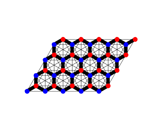
The imported model on a patch of \(5\times4\) cells (finite_system()): the honeycomb lattice of the two Wannier centres (‘a’ and ‘b’, in two colours), and every hopping in the file, drawn with a width proportional to its amplitude – the nearest-neighbour one dominates, the longer-range ones are much weaker.

fig_lat = Plot(finite_system(gra, (5, 4))).lattice(plt_hop=True, ms=12, figsize=(5.5, 4.5))

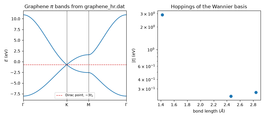
Localization: the hoppings of a maximally localized basis decay with the bond length \(|\mathbf{R} + \boldsymbol\tau_n - \boldsymbol\tau_m|\); in this file they stop after the third shell (2.84 Angstrom).

tau = gra.orbital_positions()
d = np.array([np.linalg.norm(Rc + tau[j] - tau[i]) for i, j, Rc, _ in gra._hop])
t = np.array([abs(h[3]) for h in gra._hop])
shells = np.unique(d.round(4))
print('bond lengths (Angstrom):', shells)
assert np.allclose(shells, [1.4203, 2.46, 2.8406], atol=1e-4)

bond lengths (Angstrom): [1.4203 2.46   2.8406]

The same model by neighbour order

The file is graphene with three hopping shells: built by neighbour order on the lattice read from the file, it gives the same \(H(\mathbf{k})\).

t0, t1, t2 = -2.89, 0.24, -0.27
ref = KSpace(gra.lat)
ref.set_hopping([{'n': 1, 't': t0}, {'n': 2, 't': t1}, {'n': 3, 't': t2}])
for k in np.random.default_rng(0).uniform(-3., 3., (30, 2)):
    assert np.allclose(gra.get_ham(k), ref.get_ham(k), atol=1e-12)

Closed-form energies: at \(\Gamma\), \(E_\pm = 6t_1 \pm 3|t_0 + t_2|\); at K the first- and third-neighbour sums vanish, so the Dirac point survives, shifted to \(-3t_1\).

b1, b2 = np.array(gra.rec_vec)
Gamma, K, M = np.zeros(2), (b1 - b2) / 3, b1 / 2
en_G, en_K = gra.get_bands(Gamma)[0], gra.get_bands(K)[0]
print('E(Gamma) = {} eV, E(K) = {} eV'.format(en_G.round(4), en_K.round(4)))
assert np.allclose(en_G, [6*t1 - 3*abs(t0 + t2), 6*t1 + 3*abs(t0 + t2)], atol=1e-12)
assert np.allclose(en_K, -3*t1, atol=1e-12)

E(Gamma) = [-8.04 10.92] eV, E(K) = [-0.72 -0.72] eV

Bands and hopping decay

dist, en = gra.k_path([Gamma, K, M, Gamma], nk=100)
fig, (ax1, ax2) = plt.subplots(1, 2, figsize=(9, 4))
ax1.plot(dist, en, color='C0')
for x in gra.nodes:
    ax1.axvline(x, color='k', lw=0.5)
ax1.axhline(-3*t1, color='C3', ls='--', lw=1, label='Dirac point, $-3t_1$')
ax1.set_xticks(gra.nodes)
ax1.set_xticklabels([r'$\Gamma$', 'K', 'M', r'$\Gamma$'])
ax1.set_xlim(dist[0], dist[-1])
ax1.set_ylabel('$E$ (eV)')
ax1.set_title(r'Graphene $\pi$ bands from graphene_hr.dat')
ax1.legend(fontsize=8)
ax2.semilogy(d, t, 'o')
ax2.set_xlabel(r'bond length ($\AA$)')
ax2.set_ylabel('$|t|$ (eV)')
ax2.set_title('Hoppings of the Wannier basis')
fig.tight_layout()
plt.show()