Parametrized Hamiltonians: Sweeping Without Rebuilding

A sweep over a magnetic field, a gate voltage or a dimerization usually rebuilds the model at every step: find the bonds, set the hoppings, apply the field. A value function replaces a number by a callable of the sites and of named parameters, t(site_i, site_j, **params) or onsite(site, **params). The model stores its bonds once, and get_ham() (sys.get_ham(alpha=...)) or get_ham() (ks.get_ham(k, v=...)) only re-evaluates the values. site_i and site_j are structured arrays holding every bond at once (fields 'x', 'y', 'tag', 'index'), so each function runs once per Hamiltonian, vectorized.

import numpy as np
import matplotlib.pyplot as plt

from tbkit import lattices
from tbkit.kspace import KSpace
from tbkit.plot import Plot
from tbkit.system import System

PI = np.pi

A flux sweep on a finite flake

The hopping carries the Peierls phase of a uniform field in the symmetric gauge, \(t_{ij} = -e^{i\pi\alpha(x_iy_j - x_jy_i)}\). The onsite energy is a gate voltage \(V\) that tilts the flake along \(x\). Both are set once. Each point of the sweep is a single get_ham call, and each function receives only the parameters its signature names.

N = 12
lat = lattices.square()
lat.get_lattice(n1=N, n2=N)
sys = System(lat)
sys.set_hopping([{'n': 1, 't': lambda si, sj, alpha:
                          -np.exp(1j * PI * alpha * (si['x'] * sj['y'] - sj['x'] * si['y']))}])
sys.set_onsite({'a': lambda site, V: V * (site['x'] - (N - 1) / 2) / (N - 1)})

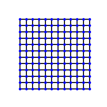
# The flake: a square of :math:`12\times12` sites with its
# nearest-neighbour bonds, which carry the Peierls phases (not drawn).
fig_lat = Plot(sys).lattice(plt_hop=True, ms=8, figsize=(4.5, 4.5))

The sweep:

alphas = np.linspace(0., 0.5, 101)
spectra = []
for alpha in alphas:
    sys.get_ham(alpha=alpha, V=0.)
    sys.get_eig()
    spectra.append(sys.en.real)
spectra = np.array(spectra)

The swept model must be the one that a full rebuild gives. With no field, it is the open square of side N, whose energies are \(-2\cos\frac{\pi m}{N+1} - 2\cos\frac{\pi l}{N+1}\). At any flux it is the model of set_magnetic_field() (same gauge). The gate shifts the spectrum’s centre of mass by the mean of the onsite energies, which is zero for this antisymmetric tilt.

c = -2 * np.cos(PI * np.arange(1, N + 1) / (N + 1))
assert np.allclose(spectra[0], np.sort((c[:, None] + c[None, :]).ravel()))
for alpha in (0.1, 1 / 3):
    ref = System(lat)
    ref.set_hopping([{'n': 1, 't': -1.}])
    ref.set_magnetic_field(alpha)
    ref.get_ham()
    ref.get_eig()
    sys.get_ham(alpha=alpha, V=0.)
    sys.get_eig()
    assert np.allclose(sys.en, ref.en)
sys.get_ham(alpha=0.1, V=1.)
sys.get_eig()
assert abs(sys.en.real.mean()) < 1e-12
assert not np.allclose(sys.en.real, ref.en.real)  # the gate does change the levels

A dimerization sweep in k-space

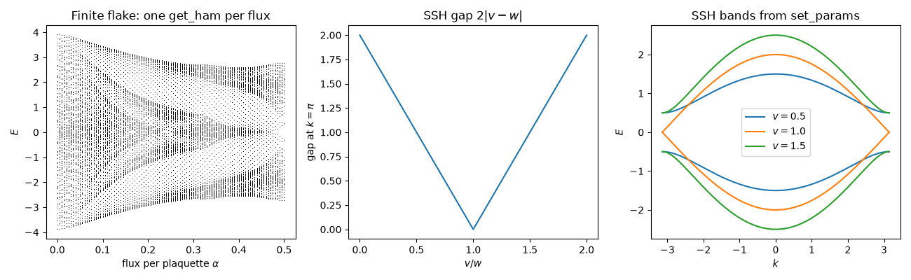
The Su-Schrieffer-Heeger chain has the intra-cell hopping \(v\) and the inter-cell hopping \(w\). Its gap, at the zone edge \(k = \pi\), is \(2|v - w|\), and it closes at the topological transition \(v = w\). Here set_params() fixes \(w\) for every method of the model, and \(v\) is passed per call.

ssh_lat = lattices.chain()
ssh_lat.unit_cell = [{'tag': 'a', 'r0': (0., 0.)}, {'tag': 'b', 'r0': (0.5, 0.)}]
ssh = KSpace(ssh_lat)
ssh.set_hopping([{'i': 0, 'j': 1, 'R': (0,), 't': lambda si, sj, v: v},
                         {'i': 1, 'j': 0, 'R': (1,), 't': lambda si, sj, w: w}])
ssh.set_params(w=1.)

vs = np.linspace(0., 2., 81)
gaps = np.array([np.ptp(np.linalg.eigvalsh(ssh.get_ham((PI,), v=v))) for v in vs])
assert np.allclose(gaps, 2 * np.abs(vs - 1.))

ks = np.linspace(-PI, PI, 201)[:, None]
bands = {}
for v in (0.5, 1., 1.5):
    ssh.set_params(v=v)
    bands[v] = ssh.get_bands(ks)
    assert np.allclose(bands[v][:, 1], np.abs(v + np.exp(1j * ks[:, 0])))

Plots

fig, axes = plt.subplots(1, 3, figsize=(13, 4))
axes[0].plot(alphas, spectra, ',k')
axes[0].set_xlabel(r'flux per plaquette $\alpha$')
axes[0].set_ylabel(r'$E$')
axes[0].set_title('Finite flake: one get_ham per flux')
axes[1].plot(vs, gaps, 'C0')
axes[1].set_xlabel(r'$v/w$')
axes[1].set_ylabel(r'gap at $k=\pi$')
axes[1].set_title(r'SSH gap $2|v-w|$')
for n, (v, en) in enumerate(bands.items()):
    axes[2].plot(ks[:, 0], en, color='C{}'.format(n), label=r'$v={}$'.format(v))
handles, labels = axes[2].get_legend_handles_labels()
axes[2].legend(handles[::2], labels[::2])
axes[2].set_xlabel(r'$k$')
axes[2].set_ylabel(r'$E$')
axes[2].set_title('SSH bands from set_params')
fig.tight_layout()