The Wannier Obstruction of Chern Bands

A band with a nonzero Chern number has no exponentially localized Wannier functions. D. J. Thouless (1984) saw the conflict: localized Wannier functions need a gauge \(|u_{\mathbf{k}}\rangle\) that is smooth and periodic over the whole Brillouin zone, and the Chern number is exactly the obstruction to one, the winding of the phase that any gauge must pick up somewhere. C. Brouder, G. Panati, M. Calandra, C. Mourougane and N. Marzari (2007) proved the converse for any number of bands: exponentially localized Wannier functions exist if and only if the Chern numbers vanish.

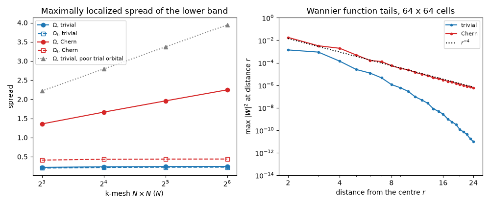
The construction makes the obstruction concrete. Projecting the band onto a trial orbital, \(A(\mathbf{k}) = \langle u_{\mathbf{k}}|g\rangle\), defines a smooth gauge wherever \(A \neq 0\). In a Chern band, every trial orbital misses the band somewhere, so \(A\) has zeros, and these zeros are vortices that no change of gauge removes. The Wannier functions then decay as a power law, and their spread \(\Omega\) grows without bound as the k-mesh (the sample) grows, while the gauge-invariant part \(\Omega_I\) stays finite.

Here tbkit.wannier.wannierize() builds the Wannier function of the lower band of the Haldane model on both sides of the transition: trivial (\(C = 0\), staggered potential \(M = 1.5\)) and Chern (\(C = 1\), \(M = 0\)).

import numpy as np
import matplotlib.pyplot as plt
from matplotlib.ticker import NullFormatter, ScalarFormatter

import tbkit.lattices as lattices
from tbkit.bridges import finite_system
from tbkit.kspace import KSpace
from tbkit.plot import Plot
from tbkit.wannier import wannierize


def haldane(t2=0.2, M=0.):
    hal = KSpace(lattices.honeycomb())
    hal.set_hopping([{'i': 0, 'j': 1, 'R': R, 't': 1.} for R in [(0, 0), (-1, 0), (0, -1)]])
    for R in [(0, 1), (-1, 0), (1, -1)]:
        hal.set_hopping([{'i': 0, 'j': 0, 'R': R, 't': 1j*t2}, {'i': 1, 'j': 1, 'R': R, 't': -1j*t2}])
    hal.set_onsite({'a': M, 'b': -M})
    return hal


trivial, chern = haldane(M=1.5), haldane(M=0.)
c_triv, c_chern = trivial.chern_number(0, 30), chern.chern_number(0, 30)
print('Chern numbers: trivial {:.3f}, Chern {:.3f}'.format(c_triv, c_chern))
assert np.isclose(c_triv, 0., atol=1e-8) and np.isclose(c_chern, 1., atol=1e-8)

Chern numbers: trivial 0.000, Chern 1.000

The lattice

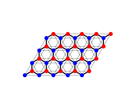
The Haldane model on a patch of \(5\times4\) cells (finite_system()), each bond drawn with a width proportional to its amplitude: the honeycomb lattice’s two sublattices (‘a’ and ‘b’, in two colours), the nearest-neighbour hopping \(t\) (thick) and the complex second-neighbour hoppings \(\pm it_2\) within each sublattice (thin), which break time-reversal symmetry. The trivial model adds the staggered mass \(\pm M\), an onsite term.

fig_lat = Plot(finite_system(chern, (5, 4))).lattice(plt_hop=True, ms=12, figsize=(5.5, 4.5))

Every projection fails somewhere

At the corners K and K’ of the Brillouin zone the lower band lies entirely on one sublattice. In the trivial phase it is the same sublattice b at both corners, and a b orbital overlaps the band everywhere. In the Chern phase the band sits on a at one corner and on b at the other, so both trial orbitals miss it at one of them: on a mesh through K and K’ (12 x 12), each projection is exactly singular.

wannierize(trivial, 0, trial=[1], nk=12)  # fine
for orbital in (0, 1):
    try:
        wannierize(chern, 0, trial=[orbital], nk=12)
        raise AssertionError('the projection should be singular')
    except ValueError:
        print('Chern band, trial orbital {}: singular projection on the 12 x 12 mesh'.format('ab'[orbital]))

Chern band, trial orbital a: singular projection on the 12 x 12 mesh
Chern band, trial orbital b: singular projection on the 12 x 12 mesh

The spread diverges with the sample

On meshes avoiding K and K’, the projection is never exactly zero, but in the Chern phase its smallest singular value falls as \(1/N\), and the minimized spread grows by about the same amount at each doubling of \(N\): like \(\log N\). In the trivial phase it converges.

meshes = np.array([8, 16, 32, 64])
runs = {name: [wannierize(model, 0, trial=[1], nk=int(n)) for n in meshes]
            for name, model in (('trivial', trivial), ('Chern', chern))}
omega = {name: np.array([wf.omega for wf in wfs]) for name, wfs in runs.items()}
omega_i = {name: np.array([wf.omega_i for wf in wfs]) for name, wfs in runs.items()}
s_min = {name: np.array([wf.min_singular_value for wf in wfs]) for name, wfs in runs.items()}
for name in runs:
    print('{:8s} Omega = {}, Omega_I = {}, min |A| = {}'.format(
        name, omega[name].round(3), omega_i[name].round(3), s_min[name].round(4)))
assert all(wf.converged for wfs in runs.values() for wf in wfs)
assert abs(omega['trivial'][-1] - omega['trivial'][-2]) < 0.005
assert np.all(np.diff(omega['Chern']) > 0.25)
assert np.all(np.abs(np.diff(omega_i['Chern'])) < 0.03)  # the gauge-invariant part converges
assert np.allclose(s_min['trivial'], s_min['trivial'][0])
assert np.all((meshes * s_min['Chern'] > 1.5) & (meshes * s_min['Chern'] < 2.))

trivial  Omega = [0.22  0.238 0.244 0.245], Omega_I = [0.203 0.219 0.224 0.226], min |A| = [0.8507 0.8507 0.8507 0.8507]
Chern    Omega = [1.356 1.664 1.958 2.246], Omega_I = [0.412 0.433 0.438 0.44 ], min |A| = [0.2012 0.1126 0.0535 0.0275]

A poor trial orbital is not the same thing. Projected onto the high-energy orbital a, even the trivial band has zeros, at K and K’: a vortex and an antivortex. Together they could be unwound, but the descent stops in the local minimum around them, and the spread grows as well. The Chern band fails the same way from either orbital; the trivial band only from the wrong one.

poor = [wannierize(trivial, 0, trial=[0], nk=int(n)).omega for n in meshes]
other = [wannierize(chern, 0, trial=[0], nk=int(n)).omega for n in meshes]
print('trivial band from orbital a: Omega = {}'.format(np.round(poor, 3)))
assert np.all(np.diff(poor) > 0.5)
assert np.allclose(other, omega['Chern'], atol=1e-6)

trivial band from orbital a: Omega = [2.217 2.791 3.369 3.943]

Exponential versus power-law tails

On the 64 x 64 sample, the trivial Wannier function decays exponentially; the Chern one only as \(|W|^2 \sim r^{-4}\), too slowly for \(\langle r^2\rangle\) to converge.

def tail(wf, radii):
    p = np.abs(wf.functions[0]) ** 2
    r = np.linalg.norm(wf.positions - wf.centers[0], axis=1)
    return np.array([p[np.abs(r - x) < 0.5].max() for x in radii])


radii = np.arange(2, 25)
tails = {name: tail(wfs[-1], radii) for name, wfs in runs.items()}
slope = np.polyfit(np.log(radii[radii >= 8]), np.log(tails['Chern'][radii >= 8]), 1)[0]
print('Chern tail: |W|^2 ~ r^{:.2f}; trivial at r = 16: {:.1e}'.format(slope, tails['trivial'][radii == 16][0]))
assert -5. < slope < -3.
assert tails['trivial'][radii == 16][0] < 1e-8 < tails['Chern'][radii == 16][0]

fig, (ax1, ax2) = plt.subplots(1, 2, figsize=(10, 4.2))
for name, color in (('trivial', 'C0'), ('Chern', 'C3')):
    ax1.semilogx(meshes, omega[name], 'o-', color=color, label=r'$\Omega$, ' + name)
    ax1.semilogx(meshes, omega_i[name], 's--', color=color, mfc='none', label=r'$\Omega_I$, ' + name)
ax1.semilogx(meshes, poor, '^:', color='gray', label=r'$\Omega$, trivial, poor trial orbital')
ax1.set_xscale('log', base=2)
ax1.set_xlabel(r'k-mesh $N \times N$ ($N$)')
ax1.set_ylabel('spread')
ax1.set_title('Maximally localized spread of the lower band')
ax1.legend(fontsize=8)
for name, color in (('trivial', 'C0'), ('Chern', 'C3')):
    ax2.loglog(radii, tails[name], 'o-', ms=3, color=color, label=name)
ax2.loglog(radii, tails['Chern'][radii == 8][0] * (radii / 8.) ** -4., 'k:', label=r'$r^{-4}$')
ax2.set_ylim(1e-14, 1)
ax2.set_xticks([2, 4, 8, 16, 24])
ax2.xaxis.set_major_formatter(ScalarFormatter())
ax2.xaxis.set_minor_formatter(NullFormatter())
ax2.set_xlabel('distance from the centre $r$')
ax2.set_ylabel(r'max $|W|^2$ at distance $r$')
ax2.set_title('Wannier function tails, 64 x 64 cells')
ax2.legend(fontsize=8)
fig.set_layout_engine('tight')
plt.show()

Chern tail: |W|^2 ~ r^-4.14; trivial at r = 16: 2.7e-09