Flat-Band Superconductivity: a Superfluid Weight Set by the Quantum Metric

A supercurrent is carried by Cooper pairs that move. In BCS theory its stiffness, the superfluid weight \(D\) (London’s \(j = -DA\)), is the density over the mass of the electrons, \(n/m\): an infinitely heavy band – a flat band – should carry no supercurrent at all, however strong the pairing. S. Peotta and P. Törmä (2015) showed that this is wrong when the flat band is made of several orbitals. An isolated flat band at filling \(\nu\), with a uniform pairing \(\Delta\) small compared with the band gaps, has (\(\hbar = e = 1\))

\[D_{\mu\nu} = 8\Delta\sqrt{\nu(1-\nu)}\int\frac{d^2\mathbf{k}}{(2\pi)^2}\,g_{\mu\nu}(\mathbf{k})\, ,\]

with \(g\) the quantum metric of the band: the pairs move by the geometry of the Bloch states, not by their dispersion, and \(D\) grows linearly with \(\Delta\) instead of saturating at \(n/m\). Since the metric bounds the Berry curvature, \(\mathrm{Tr}\,g \ge |\Omega|\), a Chern band cannot have a small superfluid weight,

\[\mathrm{Tr}\,D \ge \frac{4\Delta}{\pi}\sqrt{\nu(1-\nu)}\,|C|\, .\]

Flat bands thus superconduct, and with a critical temperature linear in the attraction – one of the explanations proposed for the superconductivity of magic-angle twisted bilayer graphene (2018).

tbkit.bdg.superfluid_weight() gets \(D\) with no flat-band approximation: the curvature of the BdG grand potential in a uniform vector potential. Below it is compared with the formula, whose metric comes from quantum_geometric_tensor().

import numpy as np
import matplotlib.pyplot as plt

import tbkit.lattices as lattices
from tbkit.bdg import superfluid_weight
from tbkit.kspace import KSpace, high_symmetry_path, magnetic_supercell

t, dimer = -1., 0.3


def lieb(delta_t):
    '''Lieb lattice, hoppings t(1 + delta_t) inside the cell, t(1 - delta_t) between cells.'''
    ks = KSpace(lattices.lieb())
    ks.set_hopping([{'i': 0, 'j': 1, 'R': (0, 0), 't': t * (1 + delta_t)},
                           {'i': 0, 'j': 1, 'R': (-1, 0), 't': t * (1 - delta_t)},
                           {'i': 0, 'j': 2, 'R': (0, 0), 't': t * (1 + delta_t)},
                           {'i': 0, 'j': 2, 'R': (0, -1), 't': t * (1 - delta_t)}])
    return ks


def metric(ks, band, nk):
    '''Integral of the quantum metric of a band over the Brillouin zone, over (2 pi)^2.'''
    _, kpts = ks.mesh_grid(nk)
    volume = abs(np.linalg.det(np.array(ks.lat.prim_vec)))
    return np.mean([ks.quantum_geometric_tensor(band, k).real for k in kpts], axis=0) / volume


def peotta_torma(delta, nu, g):
    return 8 * delta * np.sqrt(nu * (1 - nu)) * g


def filling(mu, delta, e_flat=0.):
    '''Filling of a flat band at energy e_flat: nu = (1 - xi/E)/2.'''
    xi = e_flat - mu
    return (1 - xi / np.hypot(xi, delta)) / 2

An isolated flat band

On the Lieb lattice the middle band is exactly flat, at \(E = 0\), and lives on the two edge-centre sites. Alternating the hoppings (\(t(1\pm\delta)\), Julku et al. 2016) keeps it flat and opens a gap \(2\sqrt2|t\delta|\) on both sides: an isolated flat band, with no dispersion at all but a non-zero quantum metric.

ks = lieb(dimer)
nk = 40
_, kpts = ks.mesh_grid(nk)
en = ks.get_bands(kpts)
gap = min(en[:, 2].min(), -en[:, 0].max())
assert np.ptp(en[:, 1]) < 1e-12 and abs(gap - 2 * np.sqrt(2) * abs(t * dimer)) < 1e-12
g_lieb = metric(ks, 1, nk)
print('flat band width {:.1e}, gap {:.4f}; metric integral g_xx = {:.4f}, g_xy = {:.4f}'
      .format(np.ptp(en[:, 1]), gap, g_lieb[0, 0], g_lieb[0, 1]))

points, labels = high_symmetry_path(ks.lat)
ks.k_path(points, 300)
fig_bands = ks.plot_bands(node_labels=labels, figsize=(5, 4), fs=14)

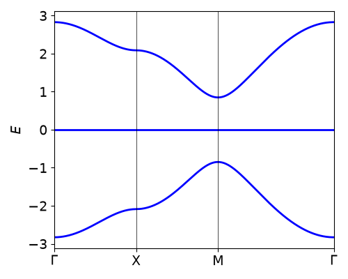
flat band width 0.0e+00, gap 0.8485; metric integral g_xx = 0.1153, g_xy = -0.0495

The superfluid weight of the flat band

At a pairing \(\Delta = 0.005|t|\), small next to the gap, the superfluid weight from the grand potential follows the formula of Peotta and Törmä to 2%, component by component, at every filling: the dome \(\sqrt{\nu(1-\nu)}\), maximal at half filling.

delta = 0.005
mus = delta * np.linspace(-3., 3., 13)
nus, d_flat = filling(mus, delta), []
for mu, nu in zip(mus, nus):
    d = superfluid_weight(ks, delta, mu=float(mu), nk=nk)
    assert np.allclose(d, peotta_torma(delta, nu, g_lieb), rtol=0.02, atol=0)
    d_flat.append(d[0, 0])
print('D_xx at half filling: {:.4e} (Peotta-Torma: {:.4e})'
      .format(d_flat[6], peotta_torma(delta, 0.5, g_lieb[0, 0])))

D_xx at half filling: 2.3019e-03 (Peotta-Torma: 2.3065e-03)

Linear in the pairing

At half filling of the flat band, \(D\) grows linearly with \(\Delta\) (to 3% up to \(\Delta = 0.05|t|\), the corrections being of order \(\Delta/\mathrm{gap}\)). With the chemical potential in the dispersive upper band, the same lattice is an ordinary BCS superconductor: \(D\) barely moves (by less than 5% while \(\Delta\) quadruples), set by the band mass, not by \(\Delta\).

deltas = np.array([0.005, 0.01, 0.02, 0.05])
d_geom = np.array([superfluid_weight(ks, float(dl), nk=nk)[0, 0] for dl in deltas])
assert np.allclose(d_geom / deltas, peotta_torma(1., 0.5, g_lieb[0, 0]), rtol=0.03, atol=0)
deltas_bcs = np.array([0.05, 0.1, 0.2])
d_bcs = np.array([superfluid_weight(ks, float(dl), mu=1.8, nk=80)[0, 0] for dl in deltas_bcs])
assert np.ptp(d_bcs) / d_bcs.mean() < 0.05 and d_bcs.min() > 5 * d_geom.max()
print('flat band: D/Delta = {}; dispersive band: D = {}'
      .format(np.round(d_geom / deltas, 4), np.round(d_bcs, 4)))

flat band: D/Delta = [0.4604 0.4594 0.4576 0.452 ]; dispersive band: D = [0.176  0.1783 0.1842]

A Chern flat band and the topological bound

Peotta and Törmä’s own model: the Harper-Hubbard model, a square lattice at flux \(1/q\) per plaquette for spin up and \(-1/q\) for spin down (time-reversal invariant, so the pairs \(\mathbf{k}\uparrow, -\mathbf{k}\downarrow\) see the same band). At \(q = 8\) the lowest Hofstadter band has \(C = 1\) and a width 800 times smaller than its gap – a nearly flat Landau level. Its metric sits just above the Chern bound, \(\int\mathrm{Tr}\,g\,d^2k/(2\pi)^2 \ge |C|/2\pi\) (within 1%), and at \(\Delta = 0.01|t|\) the superfluid weight follows the formula to 4% from 5% to 95% filling: it nearly saturates the topological bound.

q = 8
hof = magnetic_supercell(lattices.square(), [{'i': 0, 'j': 0, 'R': (1, 0), 't': t},
                                                              {'i': 0, 'j': 0, 'R': (0, 1), 't': t}], 1, q)
nk_hof = 24
_, kpts = hof.mesh_grid(nk_hof)
en_hof = hof.get_bands(kpts)
width, gap_hof = np.ptp(en_hof[:, 0]), en_hof[:, 1].min() - en_hof[:, 0].max()
chern = hof.chern_number(0, nk=nk_hof)
g_hof = metric(hof, 0, nk_hof)
assert round(chern) == 1 and gap_hof > 800 * width
assert 1 <= np.trace(g_hof) / (abs(chern) / (2 * np.pi)) < 1.01
delta_hof, e_low = 0.01, en_hof[:, 0].mean()
mus_hof = e_low + delta_hof * np.linspace(-2., 2., 9)
nus_hof = filling(mus_hof, delta_hof, e_low)
tr_d = []
for mu, nu in zip(mus_hof, nus_hof):
    d = superfluid_weight(hof, delta_hof, mu=float(mu), nk=nk_hof)
    assert np.allclose(d, peotta_torma(delta_hof, nu, g_hof), rtol=0.04, atol=1e-7)
    tr_d.append(np.trace(d))
bound = 4 * delta_hof / np.pi * np.sqrt(nus_hof * (1 - nus_hof)) * abs(chern)
assert np.all(np.abs(np.array(tr_d) / bound - 1) < 0.04)
print('Hofstadter q = {}: C = {}, width/gap = {:.1e}, Tr D / bound = {}'
      .format(q, round(chern), width / gap_hof, np.round(np.array(tr_d) / bound, 3)))

fig, axes = plt.subplots(1, 3, figsize=(14, 4))
nu_line = np.linspace(0., 1., 200)
axes[0].plot(nu_line, peotta_torma(delta, nu_line, g_lieb[0, 0]) / delta, 'k-', lw=1,
                  label=r'$8\sqrt{\nu(1-\nu)}\,\bar g_{xx}$')
axes[0].plot(nus, np.array(d_flat) / delta, 'o', c='C3', label='superfluid_weight')
axes[0].set_xlabel(r'flat-band filling $\nu$')
axes[0].set_ylabel(r'$D_{xx}/\Delta$')
axes[0].set_title(r'Lieb flat band, $\Delta = 0.005|t|$')
axes[0].legend()
axes[1].loglog(deltas, d_geom, 'o-', c='C3', label=r'flat band: $D\propto\Delta$')
axes[1].loglog(deltas_bcs, d_bcs, 's-', c='C0', label=r'dispersive band: $D\approx n/m$')
axes[1].set_xlabel(r'$\Delta/|t|$')
axes[1].set_ylabel(r'$D_{xx}$')
axes[1].set_title('geometric versus conventional')
axes[1].legend()
axes[2].plot(nu_line, 4 * delta_hof / np.pi * np.sqrt(nu_line * (1 - nu_line)), 'k-', lw=1,
                  label=r'bound $\frac{4\Delta}{\pi}\sqrt{\nu(1-\nu)}|C|$')
axes[2].plot(nus_hof, tr_d, 'o', c='C3', label=r'$\mathrm{Tr}\,D$')
axes[2].set_xlabel(r'filling $\nu$ of the $C = 1$ band')
axes[2].set_title(r'Harper-Hubbard, flux $1/{}$, $\Delta = {}|t|$'.format(q, delta_hof))
axes[2].legend()
fig.tight_layout()

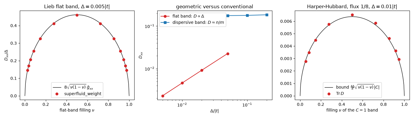
Hofstadter q = 8: C = 1, width/gap = 1.2e-03, Tr D / bound = [0.97  0.982 0.996 1.011 1.024 1.027 1.027 1.029 1.033]