
Note
Go to the end to download the full example code.
Chebyshev Time Evolution: a Wavepacket on 90,000 Sites#
Solving \(i\partial_t\psi = H\psi\) step by step, with the
Crank-Nicolson rule \((1 + iH\,dt/2)^{-1}(1 - iH\,dt/2)\) of
Propagation, needs an inverse (or a
factorization) of an \(N\times N\) matrix. Tal-Ezer and Kosloff
(J. Chem. Phys. 81, 3967 (1984)) expanded the propagator itself in
Chebyshev polynomials of the rescaled Hamiltonian
\(\tilde H = (H - b)/a\),
the recursion of the kernel polynomial method with Bessel coefficients.
\(J_m(a\Delta t)\) falls off exponentially once \(m > a\Delta t\),
so a few dozen terms beyond \(a\Delta t\) give the exact (to machine
precision) and exactly unitary propagator, whatever the step, with
nothing but sparse matrix-vector products (tbkit.kpm.time_evolution(),
or Propagation.get_propagation(..., method='chebyshev')).
Here: the exact checks (Crank-Nicolson on a small flake, and the ballistic spread of a site state on a chain), then a particle released from one site of a \(300\times300\) square lattice, clean (ballistic) and with Anderson disorder (slower than ballistic: diffusive).
import numpy as np
import matplotlib.pyplot as plt
import scipy.sparse as sparse

import tbkit.kpm as kpm
import tbkit.lattices as lattices
from tbkit.propagation import Propagation
from tbkit.system import System

t = 1.


def square(n, w=0., seed=0):
    np.random.seed(seed)
    lat = lattices.square()
    lat.get_lattice(n, n)
    sys = System(lat)  # beyond System.dense_max: neighbours from a k-d tree
    sys.set_hopping([{'n': 1, 't': t}])
    sys.set_onsite({'a': 0.})
    if w:
        sys.set_onsite_dis(w)
    sys.get_ham()
    return sys
Against Crank-Nicolson#
On a disordered \(10\times10\) flake, the Crank-Nicolson steps of
Propagation (dense, error
\(O(dt^2)\)) and the Chebyshev propagator agree to the
Crank-Nicolson error.
small = square(10, w=2.)
psi0 = np.zeros(small.lat.sites, 'c16')
psi0[55] = 1.
crank, cheb = Propagation(small.lat), Propagation(small.lat)
crank.get_propagation(small.ham, psi0, steps=400, dz=0.005)
cheb.get_propagation(small.ham, psi0, steps=400, dz=0.005, method='chebyshev')
gap = np.abs(crank.prop - cheb.prop).max()
print('Crank-Nicolson vs Chebyshev, dt = 0.005, t = 2: largest difference {:.1e}'.format(gap))
assert gap < 1e-4
assert np.allclose(np.linalg.norm(cheb.prop, axis=0), 1.)
Crank-Nicolson vs Chebyshev, dt = 0.005, t = 2: largest difference 4.2e-05
The ballistic chain#
A particle released from site 0 of a chain is \(\psi_n(\tau) = (-i)^n J_n(2t\tau)\), so \(\langle x^2\rangle = \sum_n n^2 J_n(2t\tau)^2 = 2t^2\tau^2\) exactly, as long as it has not reached the ends.
n_chain = 2001
chain = sparse.diags([np.full(n_chain - 1, t), np.full(n_chain - 1, t)], [-1, 1], format='csr')
start = np.zeros(n_chain, 'c16')
start[n_chain // 2] = 1.
tau = np.linspace(0., 300., 7)
x = np.arange(n_chain) - n_chain // 2
x2 = (np.abs(kpm.time_evolution(chain, start, tau)) ** 2 * x[:, None] ** 2).sum(axis=0)
print('<x^2> / (2 t^2 tau^2):', np.round(x2[1:] / (2 * t**2 * tau[1:]**2), 12))
assert np.allclose(x2, 2 * t**2 * tau**2, rtol=1e-10)
<x^2> / (2 t^2 tau^2): [1. 1. 1. 1. 1. 1.]
90,000 sites: ballistic and diffusive#
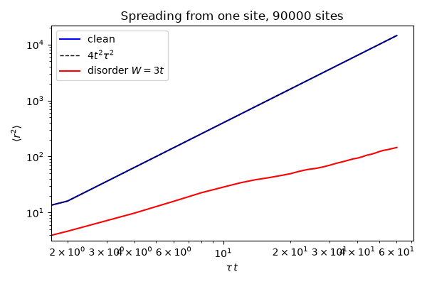
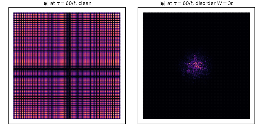
On the square lattice each direction spreads like the chain: \(\langle r^2\rangle = 4t^2\tau^2\) in the clean lattice. Disorder \(W = 3t\) scatters the particle after a mean free path; it then diffuses, \(\langle r^2\rangle \propto \tau\). A dense matrix of this size would hold \(8\times10^9\) complex numbers (130 GB).
n = 300
times = np.linspace(0., 60., 31)
spread = {}
snapshots = {}
for w in (0., 3.):
    big = square(n, w=w, seed=1)
    centre = int(np.argmin((big.lat.coor['x'] - n // 2) ** 2 + (big.lat.coor['y'] - n // 2) ** 2))
    psi_start = np.zeros(big.lat.sites, 'c16')
    psi_start[centre] = 1.
    psi = kpm.time_evolution(big.ham, psi_start, times)
    r2 = (big.lat.coor['x'] - big.lat.coor['x'][centre]) ** 2 \
        + (big.lat.coor['y'] - big.lat.coor['y'][centre]) ** 2
    spread[w] = (np.abs(psi) ** 2 * r2[:, None]).sum(axis=0)
    snapshots[w] = (big.lat.coor['x'], big.lat.coor['y'], np.abs(psi[:, -1]) ** 2)
    assert np.allclose(np.linalg.norm(psi, axis=0), 1.)
print('{} sites.'.format(n * n))
ballistic = spread[0.][1:] / (4 * t**2 * times[1:]**2)
print('clean: <r^2> / (4 t^2 tau^2) between {:.6f} and {:.6f}'.format(ballistic.min(), ballistic.max()))
assert np.allclose(spread[0.], 4 * t**2 * times**2, rtol=1e-8)  # the edges, 150 sites away, are not reached
# disordered: <r^2> grows linearly at late times (exponent close to 1, far below 2)
late = times > 30.
slope = np.polyfit(np.log(times[late]), np.log(spread[3.][late]), 1)[0]
print('disordered (W = 3t): <r^2> ~ tau^{:.2f} for tau > 30'.format(slope))
assert 0.7 < slope < 1.3

fig, ax = plt.subplots(figsize=(6, 4))
ax.plot(times, spread[0.], 'b', label='clean')
ax.plot(times, 4 * t**2 * times**2, 'k--', lw=1, label=r'$4t^2\tau^2$')
ax.plot(times, spread[3.], 'r', label='disorder $W = 3t$')
ax.set_xlabel(r'$\tau\,t$')
ax.set_ylabel(r'$\langle r^2\rangle$')
ax.set_yscale('log')
ax.set_xscale('log')
ax.legend()
ax.set_title('Spreading from one site, {} sites'.format(n * n))
fig.set_layout_engine('tight')

fig2, axes = plt.subplots(1, 2, figsize=(9, 4.4))
for axis, w, title in zip(axes, (0., 3.), ('clean', 'disorder $W = 3t$')):
    xs, ys, dens = snapshots[w]
    keep = (np.abs(xs - n // 2) < 100) & (np.abs(ys - n // 2) < 100)
    axis.scatter(xs[keep], ys[keep], c=dens[keep] ** 0.5, s=1, cmap='magma', marker='s')
    axis.set_aspect('equal')
    axis.set_title(r'$|\psi|$ at $\tau = 60/t$, ' + title)
    axis.set_xticks([])
    axis.set_yticks([])
fig2.set_layout_engine('tight')
90000 sites.
clean: <r^2> / (4 t^2 tau^2) between 1.000000 and 1.000000
disordered (W = 3t): <r^2> ~ tau^1.07 for tau > 30
Total running time of the script: (0 minutes 4.114 seconds)