
Note
Go to the end to download the full example code.
The Optical Hall Conductivity of a Disordered Chern Insulator#
The full optical conductivity tensor of a sample with no Brillouin zone, from the kernel polynomial method. With two velocities, the Kubo-Greenwood trace \(j_{ab}(E_1, E_2) = \mathrm{Tr}[v_a\,\delta(E_1-H)\,v_b\,\delta(E_2-H)]\) is complex, and
the absorptive part from the transitions at \(\hbar\omega\) and the
reactive part from all of them (Kramers-Kronig), both from the same
Chebyshev moments (tbkit.kpm.optical_conductivity() with vel_b
and part='complex'; KITE’s conductivity_optical).
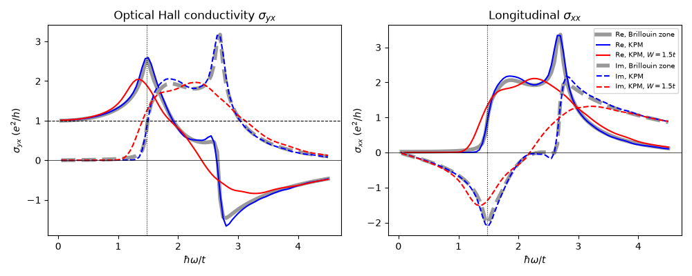
Here: a Haldane model (\(t_2 = 0.2t\), \(\phi = \pi/2\), \(M = 0.3t\)) on a \(60\times60\) torus, 7,200 sites. Below the gap, \(\mathrm{Re}\,\sigma_{yx}(\omega\to0)\) is the Chern number (TKNN), the Hall conductance that the Faraday and Kerr rotations of a thin film measure at finite frequency, and the reactive \(\mathrm{Im}\,\sigma_{xx}\) is negative (a capacitive response, no absorption). Anderson disorder leaves the low-frequency plateau at \(C\) and smears out the absorption edge.
import numpy as np
import matplotlib.pyplot as plt

import tbkit.kpm as kpm
import tbkit.lattices as lattices
import tbkit.optics as optics
from tbkit.kspace import KSpace

t, t2, m = 1., 0.2, 0.3
hal = KSpace(lattices.honeycomb())
hal.set_hopping([{'i': 0, 'j': 1, 'R': R, 't': t} for R in [(0, 0), (-1, 0), (0, -1)]])
for R in [(0, 1), (-1, 0), (1, -1)]:
    hal.set_hopping([{'i': 0, 'j': 0, 'R': R, 't': 1j * t2}, {'i': 1, 'j': 1, 'R': R, 't': -1j * t2}])
hal.set_onsite({'a': m, 'b': -m})
chern = hal.chern_number([0])
gap = 2 * (3 * np.sqrt(3) * t2 - m)  # at the Dirac point where M and the Haldane mass compete
print('Chern number of the lower band: {:.3f}, gap {:.3f}t'.format(chern, gap))
assert abs(chern - 1.) < 1e-6

n = 60
area = n * n * optics.cell_area(hal)
vx, vy = hal.finite_velocity(n, periodic=True, sparse=True)
omega = np.linspace(0.05, 4.5, 90)


def torus(w, seed=0):
    ham = hal.finite_ham(n, periodic=True, sparse=True).tolil()
    ham.setdiag(ham.diagonal() + np.random.default_rng(seed).uniform(-w / 2, w / 2, 2 * n * n))
    return ham.tocsr()


def tensor(ham):
    kw = dict(n_moments=256, n_random=24, seed=1, area=area, part="complex")
    return (kpm.optical_conductivity(ham, vy, omega, vel_b=vx, **kw),
            kpm.optical_conductivity(ham, vx, omega, **kw))
Chern number of the lower band: 1.000, gap 1.478t
The clean torus against the Brillouin zone#
Below the gap, where neither broadening (the Jackson kernel, the
Lorentzian \(\eta = 0.04t\)) matters, the torus gives the
Brillouin-zone Kubo formula of tbkit.optics.optical_conductivity():
the Hall plateau \(\mathrm{Re}\,\sigma_{yx} \to C\) as
\(\omega\to0\), rising towards the gap, and the reactive
\(\mathrm{Im}\,\sigma_{xx} < 0\), with no absorption
(\(\mathrm{Re}\,\sigma_{xx}\)) and no circular dichroism
(\(\mathrm{Im}\,\sigma_{yx}\)).
yx, xx = tensor(torus(0.))
bz_yx = optics.optical_conductivity(hal, omega, eta=0.04, nk=300, component='yx')
bz_xx = optics.optical_conductivity(hal, omega, eta=0.04, nk=300)
print('Re sigma_yx(w = {:.2f}) = {:.4f} e^2/h'.format(omega[0], yx[0].real))
assert abs(yx[0].real - chern) < 0.02
below = omega < 0.8 * gap
print('below the gap: largest deviation from the Brillouin zone {:.1%} (Re sigma_yx), {:.1%} (Im sigma_xx)'
      .format(np.max(np.abs(yx[below].real / bz_yx[below].real - 1.)),
              np.max(np.abs(xx[below & (omega > 0.2)].imag / bz_xx[below & (omega > 0.2)].imag - 1.))))
assert np.allclose(yx[below].real, bz_yx[below].real, rtol=0.03)
assert np.allclose(xx[below & (omega > 0.2)].imag, bz_xx[below & (omega > 0.2)].imag, rtol=0.05)
assert np.all(xx[below].imag < 0)
assert np.all(np.abs(xx[below].real) < 0.01) and np.all(np.abs(yx[below].imag) < 0.01)
# above the gap: absorption, and dichroism (the two circular polarizations
# are absorbed differently, Im sigma_yx != 0)
above = omega > 1.2 * gap
assert np.max(xx[above].real) > 1. and np.max(np.abs(yx[above].imag)) > 1.
Re sigma_yx(w = 0.05) = 1.0097 e^2/h
below the gap: largest deviation from the Brillouin zone 2.2% (Re sigma_yx), 3.1% (Im sigma_xx)
Disorder#
Box disorder \(W = 1.5t\), less than the gap: the Hall plateau stays at \(C\) (a topological invariant, as long as the mobility gap stays open), while the absorption edge is smeared below \(\omega = \Delta\): the disorder broadens the band edges into the gap.
yx_d, xx_d = tensor(torus(1.5))
print('disordered: Re sigma_yx(w = {:.2f}) = {:.4f} e^2/h'.format(omega[0], yx_d[0].real))
assert abs(yx_d[0].real - chern) < 0.02
# (the kernel itself rounds the clean edge over the last ~15% below the gap)
edge = (omega > 0.7 * gap) & (omega < 0.85 * gap)
print('absorption at 0.7-0.85 of the clean gap: {:.3f} (clean), {:.3f} (disordered)'.format(
      xx[edge].real.mean(), xx_d[edge].real.mean()))
assert np.all(xx[edge].real < 0.01)
assert xx_d[edge].real.mean() > 10 * xx[edge].real.mean()

fig, (ax1, ax2) = plt.subplots(1, 2, figsize=(10, 4))
for ax, (k, b, d), name in ((ax1, (yx, bz_yx, yx_d), 'yx'), (ax2, (xx, bz_xx, xx_d), 'xx')):
    for part, ls in ((np.real, '-'), (np.imag, '--')):
        label = 'Re' if part is np.real else 'Im'
        ax.plot(omega, part(b), color='0.6', lw=4, ls=ls, label=label + ', Brillouin zone')
        ax.plot(omega, part(k), 'b', ls=ls, label=label + ', KPM')
        ax.plot(omega, part(d), 'r', ls=ls, label=label + r', KPM, $W = 1.5t$')
    ax.axvline(gap, color='k', lw=0.8, ls=':')
    ax.axhline(0., color='k', lw=0.5)
    ax.set_xlabel(r'$\hbar\omega/t$')
    ax.set_ylabel(r'$\sigma_{%s}\ (e^2/h)$' % name)
ax1.axhline(chern, color='k', lw=0.8, ls='--')
ax1.set_title(r'Optical Hall conductivity $\sigma_{yx}$')
ax2.set_title(r'Longitudinal $\sigma_{xx}$')
ax2.legend(fontsize=7)
fig.set_layout_engine('tight')
disordered: Re sigma_yx(w = 0.05) = 1.0113 e^2/h
absorption at 0.7-0.85 of the clean gap: 0.003 (clean), 0.178 (disordered)
Total running time of the script: (0 minutes 21.032 seconds)