
Note
Go to the end to download the full example code.
Finite-Size Scaling of the Localization Length: MacKinnon and Kramer#
MacKinnon and Kramer (1981) measured the localization length of a long disordered bar directly, without diagonalizing anything. On a bar of cross-section \(M\times M\) the Schrödinger equation is a recurrence from one slice to the next,
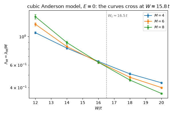
and the slowest exponential growth \(e^{n/\lambda_M}\) of a product of \(n\) of these transfer matrices sets the localization length \(\lambda_M\) of the bar. The ratio \(\Lambda_M = \lambda_M/M\) then tells the phases apart. In a metal it grows with \(M\), and in an insulator it shrinks. At the transition it does not depend on \(M\), so the curves for different widths cross at the critical disorder, \(W_c \approx 16.5\,t\) for the Anderson model of the cubic lattice (onsite energies uniform in \([-W/2, W/2]\)).
tbkit.localization.lyapunov_exponents() draws each slice, propagates
it and discards it. A bar of \(10^4\) slices never exists in memory.
import numpy as np
import matplotlib.pyplot as plt

import tbkit.lattices as lattices
from tbkit.localization import lyapunov_exponents
from tbkit.system import System
Calibration: Thouless’s weak-disorder formula#
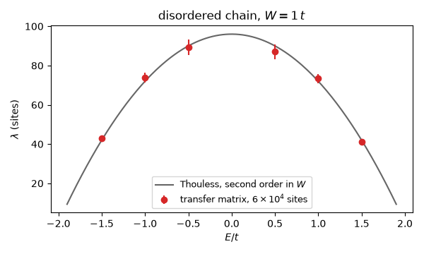
A single chain (\(M = 1\), \(h_0 = 0\), \(v = 1\)) is localized by any disorder. To second order in \(W\), Thouless’s formula gives \(1/\lambda = W^2/[24(4t^2 - E^2)]\). The band centre \(E = 0\) is left out, because the second-order result fails there (the Kappus-Wegner anomaly).
W1 = 1.
energies = np.array([-1.5, -1., -0.5, 0.5, 1., 1.5])
chain = lyapunov_exponents([[0.]], [[1.]], energies, disorder=W1, n_slices=60000, seed=1)
thouless = 24 * (4 - energies ** 2) / W1 ** 2
assert np.all(np.abs(chain.localization_length - thouless) < 3 * chain.length_error + 0.03 * thouless)

e_fine = np.linspace(-1.9, 1.9, 200)
fig1, ax = plt.subplots(figsize=(6, 3.6))
ax.plot(e_fine, 24 * (4 - e_fine ** 2) / W1 ** 2, color='0.4', label='Thouless, second order in $W$')
ax.errorbar(energies, chain.localization_length, chain.length_error, fmt='o', color='C3',
            label='transfer matrix, $6\\times10^4$ sites')
ax.set_xlabel('$E/t$')
ax.set_ylabel(r'$\lambda$ (sites)')
ax.set_title(f'disordered chain, $W = {W1:g}\\,t$', fontsize=12)
ax.legend(fontsize=9)
fig1.tight_layout()
The 3D Anderson transition#
A slice of the bar is the \(M\times M\) square lattice with periodic
boundaries, as in MacKinnon and Kramer’s own calculation (System with
periodic=True), and the coupling to the next slice is the identity.
At \(W = 12t\) the ratio \(\Lambda_M\) grows with \(M\), which
is metallic behaviour. At \(W = 20t\) it shrinks, which is
insulating. The curves for \(M = 4\) and \(M = 8\) cross in
between, near \(W_c\).
def cross_section(m):
    lat = lattices.square()
    lat.get_lattice(m, m)
    sys = System(lat, periodic=True)
    sys.set_hopping([{'n': 1, 't': 1.}])
    sys.get_ham()
    return sys.ham.toarray()


widths = (4, 6, 8)
disorders = np.array([12., 14., 16., 18., 20.])
ratio, ratio_err = {}, {}
for m in widths:
    h0 = cross_section(m)
    res = [lyapunov_exponents(h0, np.eye(m * m), 0., disorder=w, n_slices=1500 * m, seed=m, qr_every=4)
           for w in disorders]
    ratio[m] = np.array([r.localization_length[0] for r in res]) / m
    ratio_err[m] = np.array([r.length_error[0] for r in res]) / m

for n, sign in ((0, 1), (-1, -1)):       # W = 12: metal; W = 20: insulator
    gap = sign * (ratio[8][n] - ratio[4][n])
    assert gap > 3 * np.hypot(ratio_err[8][n], ratio_err[4][n]), (disorders[n], gap)
diff = ratio[8] - ratio[4]
k = np.flatnonzero(np.diff(np.sign(diff)))[0]
w_cross = disorders[k] - diff[k] * (disorders[k + 1] - disorders[k]) / (diff[k + 1] - diff[k])
assert 14. < w_cross < 19., w_cross

fig2, ax = plt.subplots(figsize=(6, 4))
for m in widths:
    ax.errorbar(disorders, ratio[m], ratio_err[m], fmt='o-', ms=4, capsize=2, label=f'$M = {m}$')
ax.axvline(16.5, color='0.6', ls='--', lw=1)
ax.text(16.6, ax.get_ylim()[1] * 0.92, r'$W_c \approx 16.5\,t$', fontsize=9, color='0.4')
ax.set_yscale('log')
ax.set_xlabel('$W/t$')
ax.set_ylabel(r'$\Lambda_M = \lambda_M/M$')
ax.set_title(f'cubic Anderson model, $E = 0$: the curves cross at $W \\approx {w_cross:.1f}\\,t$', fontsize=12)
ax.legend(fontsize=9)
fig2.tight_layout()
plt.show()
Total running time of the script: (0 minutes 18.691 seconds)