
Note
Go to the end to download the full example code.
Exact Diagonalization Against Mean Field#
Mean field (hubbard_mean_field()) replaces the
Hubbard repulsion by the potential of the average density. The check on
it is the exact ground state of a cluster small enough to diagonalize in
its full Fock space (exact_diagonalization()), on the
same hopping matrix and the same U.
The dimer. Two sites, two electrons: the exact ground state is a singlet of energy \(E_0 = (U - \sqrt{U^2 + 16t^2})/2\), and the triplet lies \(J = -E_0 \to 4t^2/U\) above it, the superexchange of the Heisenberg model.
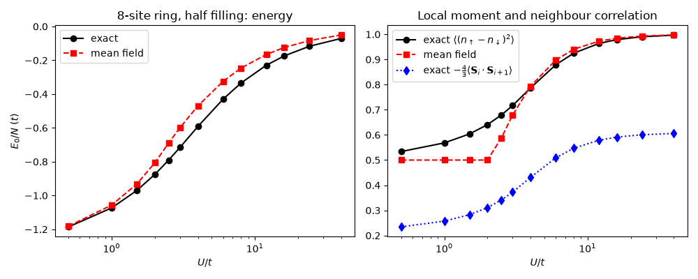
Where Hartree-Fock fails. Mean field gets a local moment only by breaking the spin symmetry, above a threshold \(U_c\): the paramagnet below, a Néel state above, neither of which is the singlet. Its energy is an upper bound (it is the energy of a Slater determinant), and at large U it misses a large part of the exchange energy, the quantum fluctuations of the spins.
import numpy as np
import matplotlib.pyplot as plt

import tbkit.lattices as lattices
from tbkit.kspace import KSpace
from tbkit.manybody import exact_diagonalization
from tbkit.meanfield import hubbard_mean_field

t = 1.
The Hubbard dimer#
dimer = np.array([[0., -t], [-t, 0.]])
us_dimer = np.array([0., 1., 4., 10., 40.])
for U in us_dimer:
    res = exact_diagonalization(dimer, 1, 1, U=U, n_states=4)
    assert np.isclose(res.energies[0], (U - np.sqrt(U ** 2 + 16 * t ** 2)) / 2)
    assert np.isclose(res.total_spin(), 0.) and np.isclose(res.spin_correlation()[0, 1], -3 / 4 * (1 - 2 * res.double_occupancy()[0]))
    triplet = exact_diagonalization(dimer, 2, 0, U=U).energies[0]   # S_z = 1, no double occupancy
    assert np.isclose(triplet, 0.) and np.isclose(res.energies[1], triplet)
J = -exact_diagonalization(dimer, 1, 1, U=40.).energies[0]
print('Dimer, U = 40t: J = {:.5f}t, 4t^2/U = {:.5f}t.'.format(J, 4 * t ** 2 / 40.))
assert abs(J / (4 * t ** 2 / 40.) - 1) < 0.01
Dimer, U = 40t: J = 0.09975t, 4t^2/U = 0.10000t.
A ring of eight sites#
Half filling, antiperiodic boundaries (a closed shell, see
finite_ham() with twist). Mean field is
started from a Néel and from a random magnetization; the lower solution
is kept. The local moment \(\langle(n_{i\uparrow} - n_{i\downarrow})^2\rangle\)
is \(\langle n_i\rangle - 2\langle n_{i\uparrow}n_{i\downarrow}\rangle\),
with the double occupancy factorized in mean field.
chain = KSpace(lattices.chain())
chain.set_hopping([{'n': 1, 't': -t}])
L = 8
ring = chain.finite_ham(L, periodic=True, twist=[np.pi]).real
neel = 0.3 * (-1) ** np.arange(L)

us = np.array([0.5, 1., 1.5, 2., 2.5, 3., 4., 6., 8., 12., 16., 24., 40.])
e_exact, e_mf, m_exact, m_mf, order_mf, s_nn = [], [], [], [], [], []
for U in us:
    ex = exact_diagonalization(ring, L // 2, L // 2, U=U)
    mf = min((hubbard_mean_field(ring, U, L, n_up=0.5 + neel, n_dn=0.5 - neel, max_iter=100000),
              hubbard_mean_field(ring, U, L, seed=0, max_iter=100000)), key=lambda r: r.energy)
    n_up, n_dn = ex.densities()
    e_exact.append(ex.energies[0])
    e_mf.append(mf.energy)
    m_exact.append(np.mean(n_up + n_dn - 2 * ex.double_occupancy()))
    m_mf.append(np.mean(mf.n_up + mf.n_dn - 2 * mf.n_up * mf.n_dn))
    order_mf.append(np.max(np.abs(mf.magnetization)))
    s_nn.append(ex.spin_correlation()[0, 1])
    assert np.isclose(ex.total_spin(), 0.) and np.allclose(n_up, 0.5) and np.allclose(n_dn, 0.5)
e_exact, e_mf, m_exact, m_mf, order_mf, s_nn = map(np.array, (e_exact, e_mf, m_exact, m_mf, order_mf, s_nn))

assert np.all(e_mf >= e_exact - 1e-9)                       # a variational upper bound
assert np.all(order_mf[us < 2.] < 1e-6) and np.all(order_mf[us > 3.] > 0.1)   # symmetry broken above U_c
assert np.all(np.diff(m_exact) > 0) and m_exact[0] > 0.5    # the exact moment grows smoothly from 1/2
assert np.allclose(m_mf[us < 2.], 0.5)                      # flat until mean field breaks the symmetry
u_c = us[np.argmax(order_mf > 1e-6)]
print('Mean-field Neel order from U = {:.1f}t; exact ground state a singlet at every U.'.format(u_c))
Mean-field Neel order from U = 2.5t; exact ground state a singlet at every U.
The Heisenberg limit: at large U the ring is a spin chain with \(J = 4t^2/U\), \(E_0 \approx J\sum_i(\langle\mathbf S_i\cdot\mathbf S_{i+1}\rangle - 1/4)\). Mean field (Néel, \(\langle S^z_iS^z_{i+1}\rangle = -1/4\)) recovers only part of it.
heisenberg = 4 * t ** 2 / us * L * (s_nn - 0.25)
print('U = 40t: E0 = {:.4f}t (exact), {:.4f}t (Heisenberg), {:.4f}t (mean field).'
      .format(e_exact[-1], heisenberg[-1], e_mf[-1]))
assert abs(e_exact[-1] / heisenberg[-1] - 1) < 2e-3
assert np.isclose(e_mf[-1], 4 * t ** 2 / us[-1] * L * (-0.5), rtol=0.02)   # J sum(-1/4 - 1/4)
assert e_mf[-1] / e_exact[-1] < 0.75

fig, axes = plt.subplots(1, 2, figsize=(10, 4))
axes[0].plot(us, e_exact / L, 'o-k', label='exact')
axes[0].plot(us, e_mf / L, 's--r', label='mean field')
axes[0].set_xscale('log')
axes[0].set_xlabel(r'$U/t$')
axes[0].set_ylabel(r'$E_0/N$ ($t$)')
axes[0].set_title('8-site ring, half filling: energy')
axes[0].legend()
axes[1].plot(us, m_exact, 'o-k', label=r'exact $\langle(n_\uparrow - n_\downarrow)^2\rangle$')
axes[1].plot(us, m_mf, 's--r', label='mean field')
axes[1].plot(us, -4 / 3 * s_nn, 'd:b', label=r'exact $-\frac{4}{3}\langle\mathbf{S}_i\cdot\mathbf{S}_{i+1}\rangle$')
axes[1].set_xscale('log')
axes[1].set_xlabel(r'$U/t$')
axes[1].set_title('Local moment and neighbour correlation')
axes[1].legend()
fig.set_layout_engine('tight')
U = 40t: E0 = -0.5637t (exact), -0.5634t (Heisenberg), -0.3997t (mean field).
Total running time of the script: (0 minutes 1.320 seconds)