The Nonlinear Hall Effect: the Berry Curvature Dipole of a Tilted Dirac Cone

A linear Hall response needs broken time-reversal symmetry: the Berry curvature \(\Omega(\mathbf{k})\) is odd in \(\mathbf{k}\) and its integral over the occupied states vanishes. Sodemann and Fu (2015) noticed that its first moment need not vanish. In a DC field (or at frequency \(\omega\)), the shifted Fermi sea carries the Hall current

\[j_a = \chi_{abc}E_bE_c\, ,\qquad \chi_{abc} = -\varepsilon_{adc}\frac{e^3\tau}{2\hbar^2(1+i\omega\tau)}D_{bd}\, ,\qquad D_a = \int\frac{d^2k}{(2\pi)^2}\sum_nf_n\,\partial_a\Omega_n\, ,\]

second order in the field, in a time-reversal-symmetric crystal with low enough symmetry: the Berry curvature dipole \(D\). It was observed in bilayer WTe₂ by Ma et al. and Kang et al. (2019).

Sodemann and Fu’s minimal model is a tilted massive Dirac cone, \(H = tk_x + v(k_x\sigma_x + k_y\sigma_y) + m\sigma_z\): the tilt leaves \(\Omega_c = -mv^2/2\varepsilon^3\) untouched but moves the Fermi surface, and to first order in \(t\), for \(\mu > |m|\),

\[D_x = -\frac{3\,t\,m\,(\mu^2 - m^2)}{8\pi\mu^4}\, ,\qquad D_y = 0\, .\]

berry_curvature_dipole() computes it on a lattice regularization of the cone (the doublers gapped by a Wilson mass), as a Fermi-surface integral over the thermal window \(-\partial f/\partial E\).

import numpy as np
import matplotlib.pyplot as plt
from scipy.integrate import quad

from tbkit.bridges import finite_system
from tbkit.kspace import KSpace, PAULI
from tbkit.lattice import Lattice
from tbkit.optics import berry_curvature_dipole
from tbkit.plot import Plot


def tilted_dirac(m, tilt, B=0.12, v=1.):
    '''tilt sin kx + v(sin kx sx + sin ky sy) + (m + B(2 - cos kx - cos ky)) sz'''
    lat = Lattice(unit_cell=[{'tag': 'a', 'r0': (0., 0.)}, {'tag': 'b', 'r0': (0., 0.)}],
                         prim_vec=[(1., 0.), (0., 1.)])
    ks = KSpace(lat)
    hop = []
    for R, s, tl in (((1, 0), 'x', tilt), ((0, 1), 'y', 0.)):
        block = -0.5j * v * PAULI[s] - 0.5 * B * PAULI['z'] - 0.5j * tl * PAULI['0']
        hop += [{'i': i, 'j': j, 'R': R, 't': complex(block[i, j])}
                     for i in range(2) for j in range(2) if block[i, j] != 0]
    ks.set_hopping(hop)
    ks.set_onsite({'a': m + 2 * B, 'b': -(m + 2 * B)})
    return ks


def sodemann_fu(mu, m, tilt):
    '''The zero-temperature dipole D_x, first order in the tilt.'''
    return -3 * tilt * m * (mu ** 2 - m ** 2) / (8 * np.pi * mu ** 4) if mu > abs(m) else 0.


def thermal(mu, T, m, tilt):
    '''The same, averaged over the thermal window -f'(E - mu).'''
    window = lambda x: 0.25 / T / np.cosh((x - mu) / (2 * T)) ** 2
    return quad(lambda x: window(x) * sodemann_fu(x, m, tilt), mu - 40 * T, mu + 40 * T,
                    points=[abs(m)], limit=200)[0]


m, tilt, T = 0.07, 0.02, 0.01
dirac = tilted_dirac(m, tilt)

The lattice

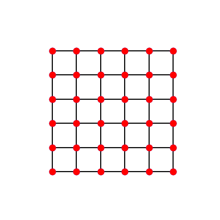
The model on \(6\times6\) cells (finite_system()): a square lattice, each site holding two orbitals (‘a’ and ‘b’, drawn on top of each other), joined by the nearest-neighbour hoppings along \(x\) and \(y\). The tilt, a small extra term on the bonds along \(x\), is too weak to show at this scale.

fig_lat = Plot(finite_system(dirac, (6, 6))).lattice(plt_hop=True, ms=10, figsize=(4.5, 4.5))

The dipole across the conduction band

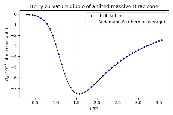
One diagonalization of the mesh gives every Fermi level. The dipole vanishes in the gap (up to a thermal tail), rises as the Fermi surface opens, and peaks near \(\mu = \sqrt2\,|m|\) (exactly there at \(T = 0\); the thermal average moves it a little), where the curvature gradient is largest on the Fermi circle. The lattice model follows the continuum formula to about 1% while the Fermi wavevector stays small.

mus = np.linspace(0.02, 0.25, 47)
dipole = berry_curvature_dipole(dirac, mus, T, nk=500)
reference = np.array([thermal(mu, T, m, tilt) for mu in mus])
inside = (mus > 0.028) & (mus < 0.181)
error = np.abs(dipole[inside, 0] / reference[inside] - 1).max()
print('largest relative deviation from Sodemann-Fu for 0.03 <= mu <= 0.18: {:.2%}'.format(error))
assert error < 0.015
# further up, the lattice (sin k, the Wilson mass) bends the cone: the
# deviation grows with the Fermi wavevector but stays small
assert np.abs(dipole[mus > 0.03, 0] / reference[mus > 0.03] - 1).max() < 0.03
assert np.abs(dipole[:, 1]).max() < 1e-12  # the mirror y -> -y forbids D_y
# deep in the gap, only the thermal tail of the conduction band is left
assert abs(dipole[0, 0]) < 0.02 * np.abs(dipole[:, 0]).max()
peak = mus[np.argmax(np.abs(dipole[:, 0]))]
print('peak at mu = {:.3f} (sqrt(2) m = {:.3f} at T = 0)'.format(peak, np.sqrt(2) * m))
assert peak == mus[np.argmax(np.abs(reference))] and abs(peak - np.sqrt(2) * m) < 0.015

largest relative deviation from Sodemann-Fu for 0.03 <= mu <= 0.18: 1.28%
peak at mu = 0.110 (sqrt(2) m = 0.099 at T = 0)

Only a tilted cone has a dipole

Without tilt the Fermi circle is centred on the curvature peak, and the dipole vanishes; reversing the tilt reverses it.

straight = berry_curvature_dipole(tilted_dirac(m, 0.), 0.12, T, nk=200)
reversed_tilt = berry_curvature_dipole(tilted_dirac(m, -tilt), 0.12, T, nk=500)
forward = berry_curvature_dipole(dirac, 0.12, T, nk=500)
assert np.allclose(straight, 0., atol=1e-12)
assert np.isclose(reversed_tilt[0], -forward[0], rtol=1e-8)

fig, ax = plt.subplots(figsize=(6, 4))
ax.plot(mus / m, 1e3 * dipole[:, 0], 'ob', ms=3, label='tbkit, lattice')
ax.plot(mus / m, 1e3 * reference, '-k', lw=1, label='Sodemann-Fu (thermal average)')
ax.axvline(np.sqrt(2), color='gray', ls=':')
ax.set_xlabel(r'$\mu / m$')
ax.set_ylabel(r'$D_x$ ($10^{-3}$ lattice constants)')
ax.set_title('Berry curvature dipole of a tilted massive Dirac cone')
ax.legend()
fig.set_layout_engine('tight')