

Note
Go to the end to download the full example code.
Three-Dimensional Topological Insulators: the Surface Dirac Cone#
In 2007 Fu, Kane and Mele, Moore and Balents, and Roy showed that the \(\mathbb{Z}_2\) topology of the quantum spin Hall effect has a 3D sequel. A time-reversal-invariant insulator in three dimensions carries four \(\mathbb{Z}_2\) indices, and the strong index \(\nu_0\) – with inversion symmetry, the product of the parities of the occupied Kramers pairs at all eight time-reversal-invariant momenta – forces every surface to host an odd number of Dirac cones: metallic, spin-momentum-locked surface states that no time-reversal-invariant perturbation can gap. Hsieh et al. saw them by photoemission in Bi1-xSbx (2008), then Xia et al. and Zhang et al. found the simplest case, a single cone, in Bi2Se3 (2009).
The model: s- and p-like orbitals with spin on a cubic lattice,
the lattice regularization of the Bi2Se3 model. The band inversion \(m < 0\) at some of the eight momenta \((0\text{ or }\pi)^3\) sets the four indices.
The photoemission picture is the surface spectral function
\(A_s(\mathbf{k}_\parallel, E)\) of the semi-infinite crystal
(surface_spectral_function(), from the Lopez
Sancho-Rubio decimation): the bulk bands projected on the surface
Brillouin zone, plus sharp lines for the states bound to the surface.
import numpy as np
import matplotlib.pyplot as plt
from mpl_toolkits.mplot3d.art3d import Line3DCollection

from tbkit.lattice import Lattice
from tbkit.kspace import KSpace, PAULI
from tbkit.system import System

cubic = [(1., 0., 0.), (0., 1., 0.), (0., 0., 1.)]
# orbitals: (s, up), (s, down), (p, up), (p, down) -> two "sites" with spin
lat = Lattice(unit_cell=[{'tag': 's', 'r0': (0., 0., 0.)}, {'tag': 'p', 'r0': (0., 0., 0.)}],
                     prim_vec=cubic)
SIGMA = [PAULI['x'], PAULI['y'], PAULI['z']]
INVERSION = np.kron(np.diag([1., -1.]), np.eye(2))  # s even, p odd


def topological_insulator(M):
    ti = KSpace(lat, spin=True)
    hops = []
    for d in range(3):
        R = tuple(int(x) for x in np.eye(3, dtype=int)[d])
        # 2 cos k_i tau_z, and sin k_i tau_x sigma_i
        hops += [{'i': 0, 'j': 0, 'R': R, 't': PAULI['0']}, {'i': 1, 'j': 1, 'R': R, 't': -PAULI['0']},
                     {'i': 0, 'j': 1, 'R': R, 't': -0.5j * SIGMA[d]},
                     {'i': 1, 'j': 0, 'R': R, 't': -0.5j * SIGMA[d]}]
    ti.set_hopping(hops)
    ti.set_onsite({'s': (M - 6) * PAULI['0'], 'p': -(M - 6) * PAULI['0']})
    return ti


k = np.array([0.3, -0.7, 1.1])
m = 2. - 2 * (3 - np.cos(k).sum())
h = m * np.kron(PAULI['z'], PAULI['0']) + sum(np.sin(k[d]) * np.kron(PAULI['x'], SIGMA[d]) for d in range(3))
assert np.allclose(topological_insulator(2.).get_ham(k), h)
The lattice#
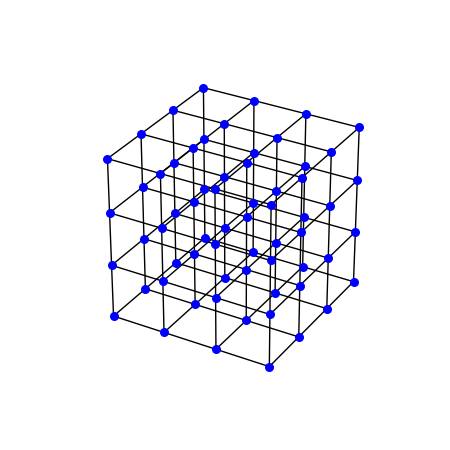
The simple cubic lattice, here \(4\times4\times4\) sites, with its nearest-neighbour bonds. Each site holds an s and a p orbital, each with spin, and every bond carries a \(4\times4\) hopping matrix that couples them (not drawn).
lat_vis = Lattice(unit_cell=[{'tag': 'a', 'r0': (0., 0., 0.)}], prim_vec=[(1., 0., 0.), (0., 1., 0.), (0., 0., 1.)])
lat_vis.get_lattice(4, 4, 4)
vis = System(lat_vis)
vis.set_hopping([{'n': 1, 't': 1.}])
pos = np.column_stack([lat_vis.coor[f] for f in 'xyz'])
bonds = np.stack([pos[vis.hop['i'].astype(int)], pos[vis.hop['j'].astype(int)]], axis=1)
fig_lat = plt.figure(figsize=(4.5, 4.5))
ax_lat = fig_lat.add_subplot(projection='3d')
ax_lat.add_collection3d(Line3DCollection(bonds, colors='k', linewidths=1))
ax_lat.scatter(*pos.T, s=30, c='b', depthshade=False)
ax_lat.set_aspect('equal')
ax_lat.set_axis_off()
The four Z2 indices#
\(m\) is \(M\) at \(\Gamma\), \(M - 4\) at the three
\(X\), \(M - 8\) at the three \(M\) and \(M - 12\) at
\(R\). The strong index counts the inverted momenta modulo 2: one
for \(0 < M < 4\) (at \(\Gamma\)), four for \(4 < M < 8\),
seven for \(8 < M < 12\). The parity criterion gives only
\(\nu_0\); z2_indices_3d() gives all four,
\((\nu_0;\nu_1\nu_2\nu_3)\), from the Wannier-centre flow on the six
time-reversal-invariant planes, without using inversion. They tell the
weak topological insulator \((0;111)\) of \(4 < M < 8\) – quantum
spin Hall layers stacked along (111), whose planes \(k_i = \pi\)
each hold one inverted momentum – from the trivial insulator, which the
strong index alone cannot.
phases = {-2.: (0, 0, 0, 0), 2.: (1, 0, 0, 0), 6.: (0, 1, 1, 1), 10.: (1, 1, 1, 1)}
for M, indices in phases.items():
    ti = topological_insulator(M)
    assert ti.parity_z2(INVERSION, [0, 1]) == indices[0]
    assert ti.z2_indices_3d([0, 1], nk=60, nk_perp=31) == indices
    print('M = {:5.1f}: (nu_0; nu_1 nu_2 nu_3) = ({}; {}{}{})'.format(M, *indices))
M =  -2.0: (nu_0; nu_1 nu_2 nu_3) = (0; 000)
M =   2.0: (nu_0; nu_1 nu_2 nu_3) = (1; 000)
M =   6.0: (nu_0; nu_1 nu_2 nu_3) = (0; 111)
M =  10.0: (nu_0; nu_1 nu_2 nu_3) = (1; 111)
The surface Dirac cone#
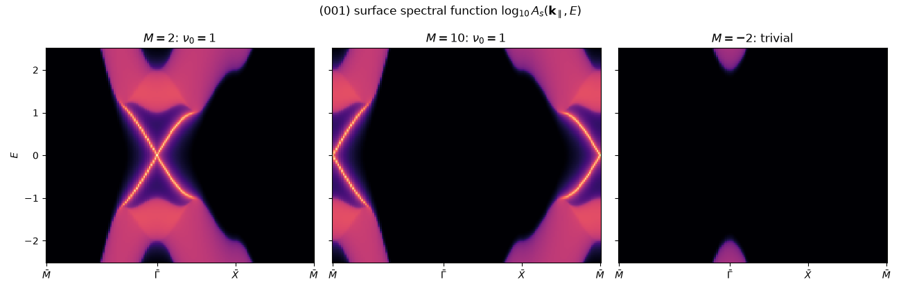
The (001) surface, along \(\bar{M}-\bar{\Gamma}-\bar{X}-\bar{M}\)
of the surface zone. Deep inside the crystal (bulk=True) there is
nothing in the gap \(|E| < 1\); on the surface of the strong
topological insulator (\(M = 2\)) a single Dirac cone crosses it,
centred at \(\bar\Gamma\), the projection of the inverted momentum,
with velocity 1.
nk = 60
corners = [np.array([np.pi, np.pi, 0.]), np.zeros(3), np.array([np.pi, 0., 0.]),
                  np.array([np.pi, np.pi, 0.])]
path = np.concatenate([np.linspace(corners[i], corners[i + 1], nk, endpoint=False)
                                     for i in range(3)] + [corners[-1:]])
dist = np.concatenate([[0.], np.cumsum(np.linalg.norm(np.diff(path, axis=0), axis=1))])
energies = np.linspace(-2.5, 2.5, 201)
eta = 0.02
gap = np.abs(energies) < 0.6  # inside the gap, beyond the broadened bulk tails

ti = topological_insulator(2.)
surface = ti.surface_spectral_function(path, energies, direction=2, eta=eta)
bulk = ti.surface_spectral_function(path, energies, direction=2, eta=eta, bulk=True)
assert bulk[:, gap].max() < 0.05
gamma = nk  # index of Gamma-bar on the path
zero = np.argmin(np.abs(energies))
assert surface[gamma, zero] > 10.
print('At Gamma-bar, E = 0: A_surface = {:.1f}, A_bulk = {:.3f}'.format(surface[gamma, zero],
                                                                                                        bulk[gamma, zero]))

# one cone: at each energy in the gap, exactly two peaks along Gamma-bar-X-bar,
# at k = |E| (and its mirror image along M-bar-Gamma-bar)
for e in (0.2, 0.4, -0.4):
    col = surface[:, np.argmin(np.abs(energies - e))]
    peaks = [i for i in range(1, len(col) - 1) if col[i] > max(col[i - 1], col[i + 1]) and col[i] > 1.]
    assert len(peaks) == 2, peaks
    k_peaks = np.abs(dist[peaks] - dist[gamma])
    assert np.allclose(k_peaks, abs(e), atol=0.06), k_peaks
print('One surface Dirac cone at Gamma-bar, velocity 1.')
At Gamma-bar, E = 0: A_surface = 28.3, A_bulk = 0.013
One surface Dirac cone at Gamma-bar, velocity 1.
Where the cone sits, and when there is none#
For \(8 < M < 12\) the inversion has moved to \(R = (\pi,\pi,\pi)\), and the cone to its projection \(\bar{M}\). In the trivial insulator (\(M = -2\)) the gap stays empty on the surface too.
surface_10 = topological_insulator(10.).surface_spectral_function(path, energies, direction=2, eta=eta)
assert surface_10[0, zero] > 10. and surface_10[gamma, zero] < 0.05
surface_triv = topological_insulator(-2.).surface_spectral_function(path, energies, direction=2, eta=eta)
assert surface_triv[:, gap].max() < 0.05
print('M = 10: the cone sits at M-bar. M = -2: no surface state in the gap.')

fig, axes = plt.subplots(1, 3, figsize=(13, 4.2), sharey=True)
titles = [r'$M = 2$: $\nu_0 = 1$', r'$M = 10$: $\nu_0 = 1$', r'$M = -2$: trivial']
ticks = [dist[0], dist[gamma], dist[2 * nk], dist[-1]]
for ax, spec, title in zip(axes, (surface, surface_10, surface_triv), titles):
    ax.pcolormesh(dist, energies, np.log10(spec.T + 1e-3), cmap='magma', vmin=-2, vmax=1.5,
                         shading='auto')
    ax.set_xticks(ticks, [r'$\bar{M}$', r'$\bar{\Gamma}$', r'$\bar{X}$', r'$\bar{M}$'])
    ax.set_title(title)
axes[0].set_ylabel('$E$')
fig.suptitle(r'(001) surface spectral function $\log_{10} A_s(\mathbf{k}_\parallel, E)$')
fig.set_layout_engine('tight')
M = 10: the cone sits at M-bar. M = -2: no surface state in the gap.
Total running time of the script: (0 minutes 4.074 seconds)