Batched and Threaded k-Space Diagonalization: the Haldane Model on 90,000 k-Points

The band and topology tools of KSpace diagonalize \(H(\mathbf{k})\) at every point of a mesh. Calling the eigensolver once per k-point spends most of its time in Python, not in LAPACK. tbkit builds all the Bloch matrices with one vectorized Bloch sum, then diagonalizes them with stacked LAPACK calls (numpy.linalg.eigh on an array of shape (nk, norb, norb)), in chunks of bounded memory. set_workers() spreads the chunks over threads (LAPACK releases the GIL).

Here: the Berry curvature of the Haldane model on a 300 x 300 mesh. The batched energies match the one-call-per-k-point loop, the Chern number does not depend on the number of threads, and the timings show the cost per k-point of each approach.

import os
import time

import numpy as np
import matplotlib.pyplot as plt
import scipy.linalg as LA

from tbkit.bridges import finite_system
from tbkit.kspace import KSpace
from tbkit.lattice import Lattice
from tbkit.plot import Plot

DX, DY = 0.5 * np.sqrt(3), 0.5
lat = Lattice(unit_cell=[{'tag': 'a', 'r0': (0., 0.)}, {'tag': 'b', 'r0': (DX, DY)}],
              prim_vec=[(2 * DX, 0.), (DX, 1.5)])
hal = KSpace(lat)
hal.set_hopping([{'i': 0, 'j': 1, 'R': R, 't': 1.} for R in [(0, 0), (-1, 0), (0, -1)]])
for R in [(1, 0), (0, 1), (1, -1)]:
    hal.set_hopping([{'i': 0, 'j': 0, 'R': R, 't': 0.2j}, {'i': 1, 'j': 1, 'R': R, 't': -0.2j}])
hal.set_onsite({'a': 0.3, 'b': -0.3})

The lattice

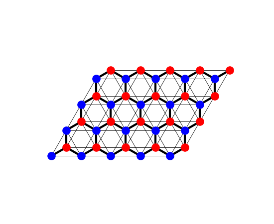
The Haldane model on a patch of \(5\times4\) cells (finite_system()), bond widths proportional to the amplitudes: the honeycomb lattice’s two sublattices (‘a’ and ‘b’, in two colours), the nearest-neighbour hopping (thick) and the complex second-neighbour hoppings \(\pm 0.2i\) (thin).

fig_lat = Plot(finite_system(hal, (5, 4))).lattice(plt_hop=True, ms=12, figsize=(5.5, 4.5))

The batched solver against one scipy call per k-point

_, ks = hal.mesh_grid(60)
t0 = time.perf_counter()
loop = np.array([LA.eigvalsh(hal.get_ham(k)) for k in ks])
t_loop = (time.perf_counter() - t0) / len(ks)
t0 = time.perf_counter()
batched = hal.mesh_bands(60)
t_batched = (time.perf_counter() - t0) / len(ks)
assert np.allclose(batched, loop)

Berry curvature on 90,000 k-points, with one thread and with several

nk = 300
t0 = time.perf_counter()
curv = hal.berry_curvature(0, nk=nk)
t_serial = (time.perf_counter() - t0) / nk ** 2
workers = min(4, os.cpu_count() or 1)
hal.set_workers(workers)
t0 = time.perf_counter()
curv_threads = hal.berry_curvature(0, nk=nk)
t_threads = (time.perf_counter() - t0) / nk ** 2
assert np.allclose(curv_threads, curv)
chern = curv.sum() / (2 * np.pi)
assert abs(chern - round(chern)) < 1e-6 and abs(round(chern)) == 1
print(f'C = {chern:.6f}')

fig, (ax0, ax1) = plt.subplots(1, 2, figsize=(10, 4))
im = ax0.imshow(curv.T * nk ** 2 / (2 * np.pi), origin='lower', extent=(0, 1, 0, 1), cmap='RdBu_r')
fig.colorbar(im, ax=ax0, label=r'$\Omega\, n_k^2 / 2\pi$')
ax0.set_xlabel(r'$k_1$ (units of $b_1$)')
ax0.set_ylabel(r'$k_2$ (units of $b_2$)')
ax0.set_title(f'Haldane model, lower band, C = {round(chern)}')
labels = ['eigvalsh\nper k-point', 'mesh_bands', 'berry_curvature\n1 thread', f'berry_curvature\n{workers} threads']
ax1.bar(labels, 1e6 * np.array([t_loop, t_batched, t_serial, t_threads]), color=['0.6', 'C0', 'C1', 'C2'])
ax1.set_ylabel(r'time per k-point ($\mu$s)')
ax1.set_title('Cost per k-point')
ax1.tick_params(axis='x', labelsize=8)
fig.tight_layout()
plt.show()

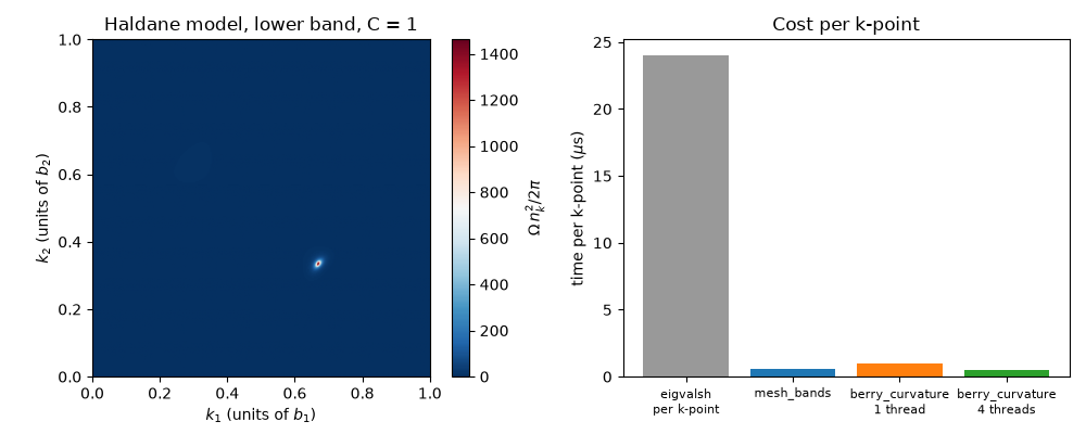
C = 1.000000