Bloch Oscillations and the Wannier-Stark Ladder

A uniform force on an electron in a periodic lattice does not produce uniform acceleration, the way it would in free space: Bloch’s 1929 argument (formalized by Wannier in 1960) shows the electron instead oscillates periodically in real space, with period \(T_B=2\pi/F\) (in units where \(\hbar=1\)). In real crystals scattering happens on a far shorter timescale than \(T_B\), which is why the effect went unobserved for over 60 years – it took artificial semiconductor superlattices (Waschke et al., 1993), with a far larger effective lattice constant, to see it directly. See History for the full historical context.

Nothing new needs to be added to tbkit for this: a linear onsite potential gradient is exactly a uniform electric field on a lattice, and System/Propagation already do the rest.

import numpy as np
import matplotlib.pyplot as plt

from tbkit.lattice import Lattice
from tbkit.system import System
from tbkit.plot import Plot
from tbkit.propagation import Propagation


N = 161
t = 1.


def tilted_chain(F, n=N):
    '''A 1D tight-binding chain with a uniform onsite potential gradient F.'''
    lat = Lattice(unit_cell=[{'tag': 'a', 'r0': (0., 0.)}], prim_vec=[(1., 0.)])
    lat.get_lattice(n1=n)
    sys = System(lat)
    sys.set_hopping([{'n': 1, 't': t}])
    sys.set_onsite({'a': 0.})
    sys.set_onsite_def({i: F*i for i in range(n)})
    sys.get_ham()
    return sys

The chain

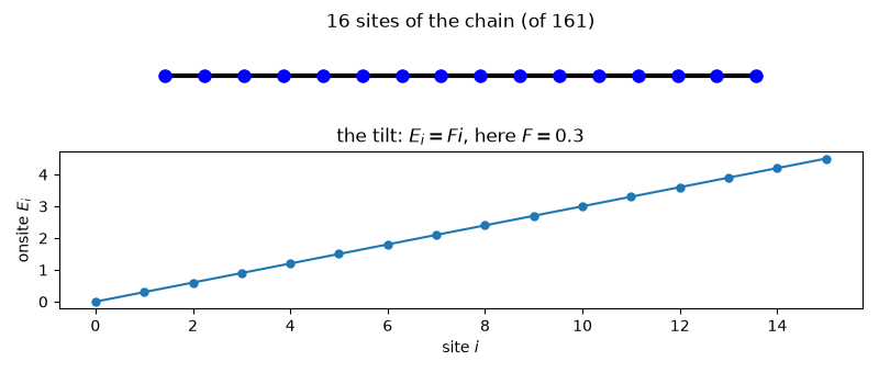
The same plain 1D chain, with the uniform force applied as a linear onsite potential gradient (again, the geometry is untouched). Only a short stretch is drawn: at the full 161 sites the markers overlap into an unreadable solid bar. What the force actually changes is not the geometry but what sits on each site, so the onsite energies are drawn below the lattice they belong to.

n_draw = 16
fig0, (ax_lat, ax_pot) = plt.subplots(2, 1, figsize=(8, 3.4),
                                                  gridspec_kw={'height_ratios': [1, 2]})
Plot(tilted_chain(F=0.3, n=n_draw)).lattice(plt_hop=True, ms=9, ax=ax_lat)
ax_lat.set_title('{} sites of the chain (of {})'.format(n_draw, N), fontsize=12)
ax_pot.plot(np.arange(n_draw), 0.3*np.arange(n_draw), 'o-', ms=5)
ax_pot.set_xlabel('site $i$')
ax_pot.set_ylabel('onsite $E_i$')
ax_pot.set_title(r'the tilt: $E_i = F i$, here $F=0.3$', fontsize=12)
fig0.tight_layout()

The Wannier-Stark ladder

The spectrum of the infinite tilted chain is exactly equally spaced, \(E_n=Fn\) – a rigorous result, not just a strong-field approximation. A finite chain reproduces it away from its two open boundaries.

F = 0.3
sys = tilted_chain(F)
sys.get_eig(eigenvec=True)
en_sorted = np.sort(sys.en.real)
spacing = np.diff(en_sorted)[20:-20]
print('Wannier-Stark ladder spacing (bulk, away from the chain ends): '
           'mean={:.5f}, std={:.2e} (expect exactly F={}).'.format(spacing.mean(), spacing.std(), F))
assert np.isclose(spacing.mean(), F, atol=1e-3)

# Its eigenstates are Wannier-Stark *localized* -- like Anderson
# localization (examples/disorder/plot_anderson_localization.py), but from
# a deterministic tilt rather than disorder, and increasingly so as the
# tilt grows.
ipr_by_F = []
for F_ in (0.05, 0.3, 1.0):
    sys_ = tilted_chain(F_)
    sys_.get_eig(eigenvec=True)
    sys_.get_ipr()
    ipr_by_F.append(sys_.ipr.mean())
    print('F={}: mean IPR = {:.4f}'.format(F_, ipr_by_F[-1]))
assert ipr_by_F[0] < ipr_by_F[1] < ipr_by_F[2]
print('Wannier-Stark localization strengthens monotonically with the tilt: OK')

Wannier-Stark ladder spacing (bulk, away from the chain ends): mean=0.30000, std=1.09e-14 (expect exactly F=0.3).
F=0.05: mean IPR = 0.0297
F=0.3: mean IPR = 0.0985
F=1.0: mean IPR = 0.2588
Wannier-Stark localization strengthens monotonically with the tilt: OK

The dynamical signature: a wavepacket oscillates instead of spreading

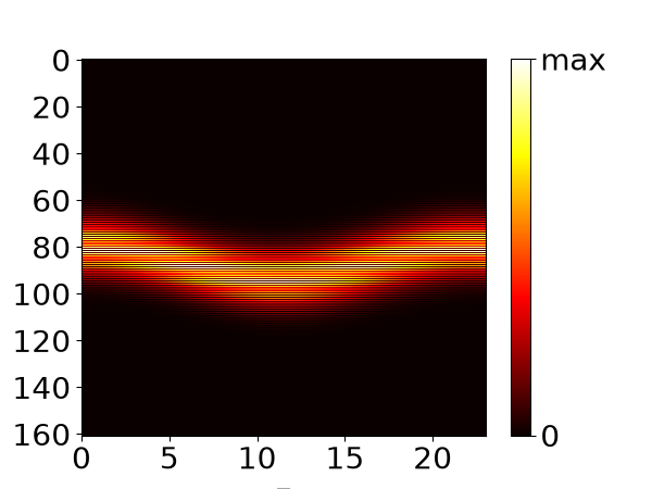
A wavepacket oscillates in real space with period \(T_B=2\pi/F\) and amplitude \(4t/F\) (the exact semiclassical result for a \(k_0=0\) wavepacket on a cosine band), instead of spreading ballistically the way it would with no tilt at all.

T_B = 2 * np.pi / F
dz = 0.02
steps = int(1.1 * T_B / dz)

x = np.arange(N)
x0 = N // 2
sigma = 8.
psi0 = np.exp(-(x - x0)**2 / (4*sigma**2)).astype('c16')
psi0 /= np.linalg.norm(psi0)

prop = Propagation(sys.lat)
prop.get_propagation(sys.ham, psi0, steps=steps, dz=dz, norm=False)

com = np.array([np.sum(x * np.abs(prop.prop[:, i])**2) for i in range(steps)]) - x0
z = dz * np.arange(steps)
amplitude = np.max(np.abs(com))
predicted_amplitude = 4 * t / F
print('Bloch oscillation amplitude: measured={:.3f}, predicted 4t/F={:.3f} '
           '(ratio={:.4f}).'.format(amplitude, predicted_amplitude, amplitude/predicted_amplitude))
assert np.isclose(amplitude, predicted_amplitude, rtol=0.01)

fig1, ax1 = plt.subplots(figsize=(6, 4.5))
ax1.plot(z / T_B, com, 'b')
ax1.axvline(1., color='k', ls='--', lw=1)
ax1.set_xlabel(r'$t / T_B$')
ax1.set_ylabel(r'$\langle x \rangle - x_0$')
ax1.set_title('Bloch oscillation: center of mass')
fig1.tight_layout()

fig2 = prop.plt_propagation_1d(prop_type='norm', figsize=(6, 4.5))

• 
• 

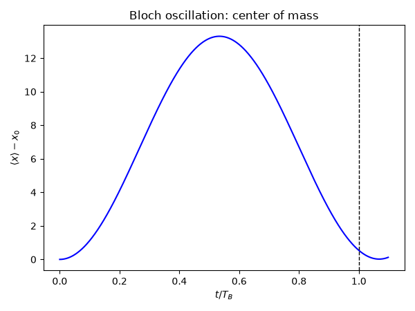
Bloch oscillation amplitude: measured=13.303, predicted 4t/F=13.333 (ratio=0.9977).