Frustrated Magnetism: the 120-Degree Order of the Triangular Hubbard Model

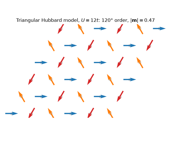
On a triangle, three antiparallel spins cannot all be satisfied: the antiferromagnet is frustrated. G. Wannier (1950) found that the Ising triangular antiferromagnet never orders; P. W. Anderson (1973) proposed that the quantum Heisenberg one is a spin liquid; the answer, settled numerically in the late 1980s (Huse and Elser 1988), is a compromise: the spins order non-collinearly, at 120 degrees from each other on the three sublattices, with zero total moment.

A collinear mean field cannot describe it. The non-collinear Hartree-Fock of tbkit.meanfield.hubbard_mean_field_noncollinear() keeps the whole spin density matrix on every site, and finds the 120-degree state of the half-filled triangular Hubbard model from random starts. At large \(U\) its energy tends to the Heisenberg limit \(-\frac{t^2}{U}\sum_{\langle ij\rangle}(1-\hat{\mathbf{m}}_i\cdot\hat{\mathbf{m}}_j)\): \(-1.5\,t^2/U\) per bond, below the \(-\frac43t^2/U\) of the best collinear (up-up-down) state.

import numpy as np
import matplotlib.pyplot as plt

import tbkit.lattices as lattices
from tbkit.kspace import KSpace
from tbkit.meanfield import hubbard_mean_field_noncollinear
from tbkit.higher_order import flake_positions
from tbkit.plot import Plot
from tbkit.system import System

tri = KSpace(lattices.triangular())
tri.set_hopping([{'i': 0, 'j': 0, 'R': (1, 0), 't': 1.}, {'i': 0, 'j': 0, 'R': (0, 1), 't': 1.},
                         {'i': 0, 'j': 0, 'R': (1, -1), 't': 1.}])

The triangular lattice

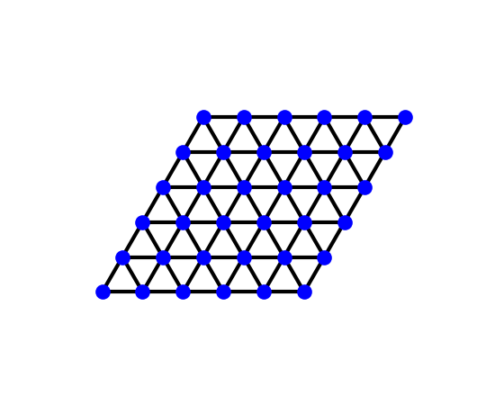
One site per unit cell, six nearest neighbours, and every elementary plaquette a triangle: no two-sublattice (Neel) pattern fits on it.

patch = lattices.triangular()
patch.get_lattice(n1=6, n2=6)
vis = System(patch)
vis.set_hopping([{'n': 1, 't': 1.}])
fig_lat = Plot(vis).lattice(plt_hop=True, ms=12, figsize=(5.5, 4.5))

The 120-degree state and its energy

n = 3
h = tri.finite_ham(n, periodic=True).real
bonds = 3 * n * n
cells = np.array([(i, j) for j in range(n) for i in range(n)])
sub = (cells[:, 0] - cells[:, 1]) % 3
for U in (12., 40.):
    best = min((hubbard_mean_field_noncollinear(h, U, n * n, seed=s) for s in range(3)),
                   key=lambda r: r.energy)
    u = best.magnetization / np.linalg.norm(best.magnetization, axis=1)[:, None]
    assert np.allclose((u @ u.T)[np.abs(h) > 0], -0.5, atol=1e-4)
    assert np.allclose(best.total_spin, 0., atol=1e-6)
    mag = np.zeros((n * n, 3))
    mag[:, 2] = np.where(sub == 0, -0.3, 0.3)
    uud = hubbard_mean_field_noncollinear(h, U, n * n, magnetization=mag)
    assert best.energy < uud.energy
    print('U = {:4.0f}: |m| = {:.3f}, E U/t^2 per bond: 120 deg {:.3f}, up-up-down {:.3f}'.format(
        U, np.linalg.norm(best.magnetization[0]), best.energy * U / bonds, uud.energy * U / bonds))
assert abs(best.energy * U / bonds + 1.5) < 0.03 and abs(uud.energy * U / bonds + 4 / 3) < 0.03

U =   12: |m| = 0.476, E U/t^2 per bond: 120 deg -1.359, up-up-down -1.271
U =   40: |m| = 0.497, E U/t^2 per bond: 120 deg -1.485, up-up-down -1.329

The moments on a 6 x 6 torus

n = 6
h = tri.finite_ham(n, periodic=True).real
res = min((hubbard_mean_field_noncollinear(h, 12., n * n, seed=s) for s in range(2)),
              key=lambda r: r.energy)
m = res.magnetization
# the moments are coplanar: rotate their plane onto the xy plane
normal = np.linalg.svd(m)[2][-1]
assert np.allclose(m @ normal, 0., atol=1e-5)
e1 = m[0] / np.linalg.norm(m[0])
e2 = np.cross(normal, e1)
pos = flake_positions(tri, n)
u = m / np.linalg.norm(m, axis=1)[:, None]
assert np.allclose((u @ u.T)[np.abs(h) > 0], -0.5, atol=1e-4)

fig, ax = plt.subplots(figsize=(6, 5))
ax.scatter(pos[:, 0], pos[:, 1], c='0.8', s=40, zorder=1)
angle = np.arctan2(m @ e2, m @ e1)
sector = np.rint(angle / (2 * np.pi / 3)).astype(int) % 3  # three sublattices
colors = np.array(['C0', 'C1', 'C3'])[sector]
ax.quiver(pos[:, 0], pos[:, 1], m @ e1, m @ e2, color=colors, pivot='middle', scale=6, zorder=2)
ax.set_aspect('equal')
ax.axis('off')
ax.set_title(r'Triangular Hubbard model, $U = 12t$: 120° order, $|\mathbf{{m}}| = {:.2f}$'.format(
    np.linalg.norm(m[0])))
fig.tight_layout()