The Peierls Substitution: Flux Through the Plaquettes, in Any Gauge

R. Peierls (1933) put a magnetic field on a lattice by attaching to each hopping the line integral of the vector potential along its bond,

\[t_{ij} \to t_{ij}\,e^{i\phi_{ij}}\, ,\qquad \phi_{ij} = \frac{2\pi}{\Phi_0}\int_{\mathbf{r}_i}^{\mathbf{r}_j}\mathbf{A}\cdot d\mathbf{l}\, .\]

The individual phases depend on the gauge, but the product of the phases around any closed loop does not: it is \(e^{2\pi i\Phi/\Phi_0}\), with \(\Phi\) the flux through the loop. Everything physical – spectra, densities, currents – depends on those loop products only, so two gauges of the same field give unitarily equivalent Hamiltonians.

set_magnetic_field() applies the symmetric gauge \(\mathbf{A} = \frac B2(-y, x)\); set_peierls_phase() any other.

import numpy as np
import matplotlib.pyplot as plt

import tbkit.lattices as lattices
from tbkit.plot import Plot
from tbkit.system import System

alpha = 0.07  # flux quanta per unit area


def flake(lattice, n):
    lat = getattr(lattices, lattice)()
    lat.get_lattice(n, n)
    lat.center()
    sys = System(lat)
    sys.set_hopping([{'n': 1, 't': 1.}])
    return sys


def loop_phase(ham, loop):
    '''Phase of the product of the hoppings around a closed loop of sites.'''
    prod = np.prod([ham[a, b] for a, b in zip(loop, loop[1:] + loop[:1])])
    return np.angle(prod)

The two flakes

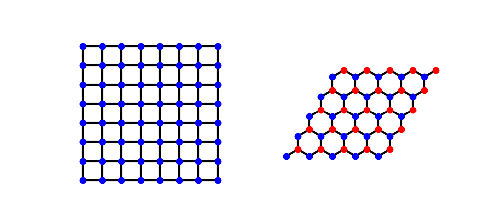
A square flake of \(8\times8\) sites and a honeycomb flake of \(5\times5\) cells (sublattices ‘a’ and ‘b’ in two colours), each with its nearest-neighbour bonds. The field enters only through the phases of these hoppings.

fig_lat, axes_lat = plt.subplots(1, 2, figsize=(10, 4.5))
Plot(flake('square', 8)).lattice(plt_hop=True, ms=10, ax=axes_lat[0])
Plot(flake('honeycomb', 5)).lattice(plt_hop=True, ms=10, ax=axes_lat[1])

<Figure size 1000x450 with 2 Axes>

The flux through every square plaquette

sys = flake('square', 8)
sys.set_magnetic_field(alpha)
sys.get_ham()
ham = sys.ham.toarray()
x, y = sys.lat.coor['x'], sys.lat.coor['y']
index = {(round(a, 6), round(b, 6)): i for i, (a, b) in enumerate(zip(x, y))}
phases = []
for (a, b), i in index.items():
    corners = [(a, b), (a + 1, b), (a + 1, b + 1), (a, b + 1)]
    keys = [(round(c, 6), round(d, 6)) for c, d in corners]
    if all(k in index for k in keys):
        phases.append(loop_phase(ham, [index[k] for k in keys]))
print('{} plaquettes: loop phase {:.6f} for every one (2 pi alpha = {:.6f}).'
          .format(len(phases), np.mean(phases), 2*np.pi*alpha))
assert np.allclose(phases, 2*np.pi*alpha)

49 plaquettes: loop phase 0.439823 for every one (2 pi alpha = 0.439823).

Another gauge, the same physics

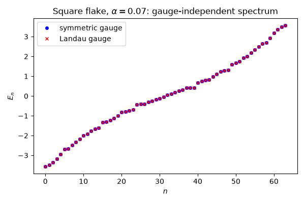
The Landau gauge \(\mathbf{A} = B(0, x)\), and any gauge transformation \(\phi_{ij}\to\phi_{ij} + \chi_j - \chi_i\), give the same spectrum.

landau = flake('square', 8)
landau.set_peierls_phase(lambda xi, yi, xj, yj: 2*np.pi*alpha*(yj - yi)*(xi + xj)/2)
landau.get_ham()
chi = np.random.default_rng(0).uniform(0, 2*np.pi, landau.lat.sites)
gauged = flake('square', 8)
index_of = {(round(a, 6), round(b, 6)): i for i, (a, b) in enumerate(zip(gauged.lat.coor['x'], gauged.lat.coor['y']))}
gauged.set_peierls_phase(lambda xi, yi, xj, yj: 2*np.pi*alpha*(yj - yi)*(xi + xj)/2
                                   + chi[[index_of[(round(a, 6), round(b, 6))] for a, b in zip(xj, yj)]]
                                   - chi[[index_of[(round(a, 6), round(b, 6))] for a, b in zip(xi, yi)]])
gauged.get_ham()
spectra = [np.linalg.eigvalsh(s.ham.toarray()) for s in (sys, landau, gauged)]
assert np.allclose(spectra[0], spectra[1]) and np.allclose(spectra[0], spectra[2])
print('Symmetric gauge, Landau gauge, and a random gauge transformation: identical spectra.')

Symmetric gauge, Landau gauge, and a random gauge transformation: identical spectra.

On the honeycomb lattice: the flux through a hexagon

hon = flake('honeycomb', 5)
hon.set_magnetic_field(alpha)
hon.get_ham()
h = hon.ham.toarray()
# every complete hexagon: six sites at distance 1 from a hexagon centre,
# which lies one unit above each site
xy = np.stack([hon.lat.coor['x'], hon.lat.coor['y']], axis=1)
found = []
for c in xy:
    ring = np.flatnonzero(np.isclose(np.linalg.norm(xy - (c + [0., 1.]), axis=1), 1.))
    if len(ring) == 6:
        angles = np.arctan2(*(xy[ring] - (c + [0., 1.]))[:, ::-1].T)
        found.append(list(ring[np.argsort(angles)]))
hex_area = 3 * np.sqrt(3) / 2
phase = [loop_phase(h, loop) for loop in found]
print('{} hexagons: loop phase {:.6f} (2 pi alpha x hexagon area = {:.6f}).'
          .format(len(found), np.mean(phase), 2*np.pi*alpha*hex_area))
assert len(found) > 0 and np.allclose(phase, 2*np.pi*alpha*hex_area)

fig, ax = plt.subplots(figsize=(6, 4))
ax.plot(spectra[0], 'ob', ms=4, label='symmetric gauge')
ax.plot(spectra[1], 'xr', ms=5, label='Landau gauge')
ax.set_xlabel('$n$')
ax.set_ylabel('$E_n$')
ax.legend()
ax.set_title(r'Square flake, $\alpha = {}$: gauge-independent spectrum'.format(alpha))
fig.set_layout_engine('tight')

16 hexagons: loop phase 1.142694 (2 pi alpha x hexagon area = 1.142694).