The Inverse Participation Ratio and Multifractal Wave Functions

Bell and Dean (1970) measured how many atoms of a glass take part in a vibration with the participation ratio; its inverse,

\[\mathrm{IPR}_n = \frac{\sum_i|\psi_i^{(n)}|^4}{\left(\sum_i|\psi_i^{(n)}|^2\right)^2}\, ,\]

became the standard probe of localization (get_ipr()). Its value alone says little; its scaling with the system size \(N\) says everything. Wegner (1980) generalized it to every moment,

\[P_q = \sum_i |\psi_i|^{2q} \sim N^{-D_q(q-1)}\, ,\]

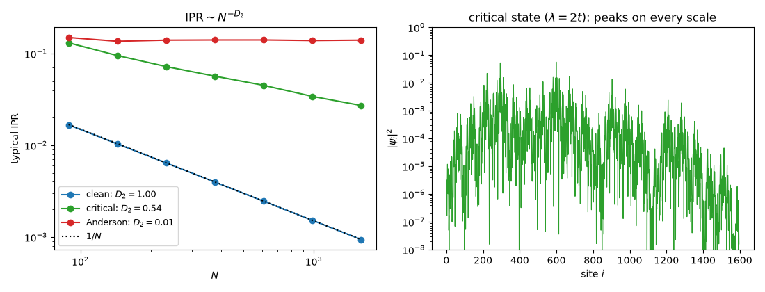
and showed that at a localization transition the exponents \(D_q\) are neither 1 (extended: \(|\psi_i|^2 \sim 1/N\) everywhere) nor 0 (localized: a few sites carry the weight), but fractal dimensions that change with \(q\). The wave function is multifractal: its strong and weak peaks fill the lattice with different dimensions.

Three 1D chains show the three cases: a clean chain, an Anderson chain, and the Harper (Aubry-André) chain at its critical point \(\lambda = 2t\).

import numpy as np
import matplotlib.pyplot as plt

import tbkit.lattices as lattices
from tbkit.plot import Plot
from tbkit.system import System


BETA = (np.sqrt(5) - 1) / 2
SIZES = [89, 144, 233, 377, 610, 987, 1597]


def chain(n, model):
    lat = lattices.chain()
    lat.get_lattice(n1=n)
    sys = System(lat)
    sys.set_hopping([{'n': 1, 't': 1.}])
    if model == 'critical':
        sys.set_onsite({'a': lambda site: 2. * np.cos(2 * np.pi * BETA * site['index'] + 0.3)})
    else:
        sys.set_onsite({'a': 0.})
    if model == 'Anderson':
        state = np.random.get_state()
        np.random.seed(0)
        sys.set_onsite_dis(alpha=1.5)
        np.random.set_state(state)
    sys.get_ham()
    sys.get_eig(eigenvec=True)
    sys.get_ipr()
    return sys


def moment(sys, q):
    r'''Typical (geometric-mean) P_q over all the eigenstates.'''
    return np.exp(np.mean(np.log(np.sum(sys.intensity**q, axis=0))))

The chain

All three models share one open chain with uniform nearest-neighbour hopping; clean, critical (Aubry-Andre at \(\lambda = 2t\)) and Anderson differ only in their onsite energies.

fig_lat = Plot(chain(12, 'clean')).lattice(plt_hop=True, ms=12, figsize=(8, 1.2))

The IPR is the q = 2 moment

get_ipr is the definition above, applied to every eigenvector.

sys = chain(144, 'critical')
psi2 = np.abs(sys.rn)**2
assert np.allclose(sys.ipr, np.sum(psi2**2, axis=0) / np.sum(psi2, axis=0)**2)

Scaling with the size: the exponents \(D_q\)

\(D_q\) is minus the slope of \(\ln P_q\) against \(\ln N\), divided by \(q - 1\).

qs = (2, 3, 4)
models = ('clean', 'critical', 'Anderson')
moments = {m: np.array([[moment(s, q) for q in qs] for s in (chain(n, m) for n in SIZES)]).T for m in models}
dq = {m: np.array([-np.polyfit(np.log(SIZES), np.log(p), 1)[0] / (q - 1)
                   for q, p in zip(qs, moments[m])]) for m in models}
for m in models:
    print('{:>8}: D_2, D_3, D_4 = {}'.format(m, np.round(dq[m], 3)))
assert np.allclose(dq['clean'], 1., atol=0.05)  # extended
assert np.allclose(dq['Anderson'], 0., atol=0.05)  # localized
assert np.all((0.3 < dq['critical']) & (dq['critical'] < 0.7))  # fractal ...
assert dq['critical'][0] - dq['critical'][-1] > 0.05  # ... and multifractal: D_q falls with q
print('D_q = 1 (clean), 0 (Anderson), and decreasing between 0.3 and 0.7 at the critical point: OK')

   clean: D_2, D_3, D_4 = [0.997 0.997 0.997]
critical: D_2, D_3, D_4 = [0.538 0.477 0.446]
Anderson: D_2, D_3, D_4 = [0.012 0.012 0.013]
D_q = 1 (clean), 0 (Anderson), and decreasing between 0.3 and 0.7 at the critical point: OK

The three scalings, and a critical wave function

fig, axes = plt.subplots(1, 2, figsize=(11, 4.2))
for m, c in zip(models, ('C0', 'C2', 'C3')):
    axes[0].loglog(SIZES, moments[m][0], 'o-', c=c, label=r'{}: $D_2 = {:.2f}$'.format(m, dq[m][0]))
axes[0].loglog(SIZES, 1.5 / np.array(SIZES), 'k:', label='$1/N$')
axes[0].set_xlabel('$N$')
axes[0].set_ylabel('typical IPR')
axes[0].legend(fontsize=9)
axes[0].set_title(r'$\mathrm{IPR} \sim N^{-D_2}$')
sys = chain(SIZES[-1], 'critical')
axes[1].semilogy(sys.intensity[:, SIZES[-1] // 2], 'C2', lw=0.8)
axes[1].set_ylim(1e-8, 1)
axes[1].set_xlabel('site $i$')
axes[1].set_ylabel(r'$|\psi_i|^2$')
axes[1].set_title(r'critical state ($\lambda = 2t$): peaks on every scale')
fig.tight_layout()