The Bogoliubov-de Gennes Equations: Andreev Bound States

P.-G. de Gennes (1966) wrote the BCS mean field site by site: a quasiparticle is a two-component wave function \((u_i, v_i)\), an electron and a hole, solving

\[\begin{split}\begin{pmatrix} h - \mu & \Delta \\ \Delta^\dagger & -(h - \mu)^T\end{pmatrix} \begin{pmatrix} u \\ v\end{pmatrix} = E\begin{pmatrix} u \\ v\end{pmatrix}\, ,\end{split}\]

with a pairing potential \(\Delta_i\) free to vary in space. On a clean lattice it gives back the BCS spectrum \(E_k = \pm\sqrt{\xi_k^2 + |\Delta|^2}\); its power is everything that is not clean: interfaces, junctions, vortices and impurities. The classic case is a junction. An electron in a normal region between two superconductors is Andreev-reflected as a hole at each interface, and the round trips quantize into Andreev bound states inside the gap (de Gennes and Saint-James, 1963). Where the two superconductors meet with a phase difference \(\varphi\) and no normal region, a single bound state sits at \(E = \Delta|\cos(\varphi/2)|\) (Kulik and Omelyanchuk, 1977): the current it carries is the Josephson current.

bdg_ham() builds the BdG matrix of any spinful real-space Hamiltonian (here an OrbitalSystem chain) and a pairing such as pairing_s_wave(), scaled site by site.

import numpy as np
import matplotlib.pyplot as plt
import scipy.sparse as sparse

import tbkit.lattices as lattices
from tbkit.bdg import bdg_ham, pairing_s_wave, particle_hole
from tbkit.orbital import OrbitalSystem
from tbkit.plot import Plot
from tbkit.system import System

t, delta = -1., 0.1  # half filling: coherence length 2|t|/delta = 20 sites


def chain(n, periodic=False):
    lat = lattices.chain()
    lat.get_lattice(n)
    sys = OrbitalSystem(lat, spin=True, periodic=periodic)
    sys.set_hopping([{'n': 1, 't': t}])
    sys.get_ham()
    return sys


def junction(n_s, length, phi):
    '''BdG spectrum of an S-N-S chain: two superconductors of n_s sites,
    phases 0 and phi, around a normal region of the given length.'''
    n = 2 * n_s + length
    gap = np.zeros(n, 'c16')
    gap[:n_s], gap[n_s + length:] = delta, delta * np.exp(1j * phi)
    pairing = sparse.diags(np.repeat(gap, 2)) @ pairing_s_wave(n, 1.)
    return np.linalg.eigvalsh(bdg_ham(chain(n).ham, pairing).toarray())

The lattice

Every model below lives on a chain with one site per cell and a nearest-neighbour hopping \(t\), each site holding a spin-1/2 orbital; the s-wave pairing \(\Delta\) binds the two spins of a site.

patch = lattices.chain()
patch.get_lattice(n1=10)
vis = System(patch)
vis.set_hopping([{'n': 1, 't': t}])
fig_lat = Plot(vis).lattice(plt_hop=True, ms=12, figsize=(7, 1.2))

A clean superconductor: the BCS spectrum

On a ring of 40 sites, the 160 BdG energies are \(\pm E_k\), each twice (spin), and the matrix anticommutes with the particle-hole operator \(\tau_x\mathcal{K}\).

n = 40
ham_bdg = bdg_ham(chain(n, periodic=True).ham, pairing_s_wave(n, delta)).toarray()
k = 2 * np.pi * np.arange(n) / n
e_k = np.sqrt((2 * t * np.cos(k)) ** 2 + delta ** 2)
assert np.allclose(np.linalg.eigvalsh(ham_bdg), np.sort(np.concatenate([e_k, e_k, -e_k, -e_k])))
tau_x = particle_hole(2 * n)
assert np.allclose(tau_x @ ham_bdg.conj() @ tau_x, -ham_bdg)
print('Ring: BdG spectrum = +-sqrt(xi_k^2 + Delta^2); smallest |E| = {:.3f} = Delta.'
          .format(np.abs(np.linalg.eigvalsh(ham_bdg)).min()))

Ring: BdG spectrum = +-sqrt(xi_k^2 + Delta^2); smallest |E| = 0.100 = Delta.

A phase jump: the Kulik-Omelyanchuk level

Two superconductors of 200 sites each, in direct contact, with a phase difference. One Andreev level (twice, for spin) leaves the continuum and follows the Kulik-Omelyanchuk law.

phis = np.linspace(0., 0.95 * np.pi, 12)
andreev = []
for phi in phis:
    en = junction(200, 0, phi)
    andreev.append(np.sort(en[en > 0])[0])
andreev = np.array(andreev)
assert np.allclose(andreev, delta * np.abs(np.cos(phis / 2)), atol=0.02 * delta)
print('Phase jump: Andreev level within {:.1%} of Delta |cos(phi/2)|.'
          .format(np.max(np.abs(andreev / delta - np.abs(np.cos(phis / 2))))))

Phase jump: Andreev level within 1.4% of Delta |cos(phi/2)|.

A normal region: de Gennes-Saint-James states

At equal phases, a normal region of growing length L traps more and more Andreev levels below the gap, ever closer to zero energy.

lengths = [0, 20, 50, 100, 200]
levels, counts = [], []
for length in lengths:
    en = junction(200, length, 0.)
    pos = np.sort(en[en > 0])
    levels.append(pos[pos < delta])
    counts.append(int(np.sum(pos < 0.99 * delta)))
print('L =', lengths, '-> bound states below the gap:', counts)
assert counts[0] == 0 and np.all(np.diff(counts) >= 0) and counts[-1] >= 10
assert np.all(np.diff([lv[0] for lv in levels[1:]]) < 0)

fig, axes = plt.subplots(1, 2, figsize=(10, 4))
fine = np.linspace(0, np.pi, 200)
axes[0].plot(fine / np.pi, np.abs(np.cos(fine / 2)), '-k', label=r'$|\cos(\varphi/2)|$')
axes[0].plot(phis / np.pi, andreev / delta, 'or', label='BdG, phase jump')
axes[0].set_xlabel(r'$\varphi/\pi$')
axes[0].set_ylabel(r'$E/\Delta$')
axes[0].legend()
for length, lv in zip(lengths, levels):
    axes[1].plot(np.full(len(lv), length), lv / delta, '_b', ms=14, mew=2)
axes[1].axhline(1., color='k', ls='--')
axes[1].set_xlabel('length L of the normal region (sites)')
axes[1].set_ylabel(r'subgap levels $E/\Delta$')
axes[1].set_title('de Gennes-Saint-James states')
fig.set_layout_engine('tight')

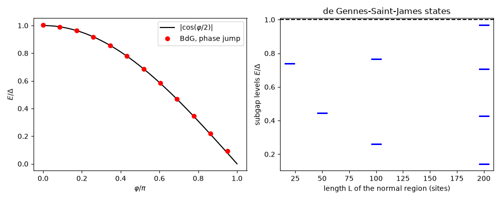
L = [0, 20, 50, 100, 200] -> bound states below the gap: [0, 4, 4, 8, 16]