Andreev Reflection: the BTK Conductance of a Normal-Superconductor Junction

An electron from a normal metal, with an energy inside the superconducting gap \(\Delta\), cannot enter the superconductor alone. Andreev (1964) showed that it is retro-reflected as a hole while a Cooper pair enters the condensate, which carries a charge \(2e\) across the interface. Blonder, Tinkham and Klapwijk (BTK, 1982) turned this into the conductance of a normal-superconductor (NS) junction with a barrier of strength \(Z\),

\[G_{NS} = \frac{e^2}{h}\left(1 + R_{he} - R_{ee}\right)\, ,\]

with \(R_{he}\) the Andreev and \(R_{ee}\) the normal reflection probabilities. A clean interface (\(Z = 0\)) doubles the conductance in the gap. A tunnel barrier (\(Z \gg 1\)) suppresses it and leaves the superconductor’s density of states, peaked at \(E = \Delta\).

The Bogoliubov-de Gennes chain has an electron and a hole orbital per site. The normal lead conserves the electron-hole charge \(\tau_z\), so add_lead(..., conservation_law=tau_z) splits its modes into electrons (block 1) and holes (block 0), and the scattering matrix (smatrix()) gives \(R_{he}\) and \(R_{ee}\) as blocks. The superconducting lead has no such law.

import numpy as np
import matplotlib.pyplot as plt

from tbkit.lattice import Lattice
from tbkit.plot import Plot
from tbkit.system import System
from tbkit.transport import Transport


gap, n = 0.01, 20
tau_z = np.diag([1., -1.])
pairing = np.array([[0., 1.], [1., 0.]])


def ns_junction(barrier):
    r'''
    A chain at half filling (t = 1): normal on the left, s-wave
    superconducting on the right, with an onsite barrier U at the interface.
    '''
    ham = np.kron(np.eye(n, k=1) + np.eye(n, k=-1), -tau_z)
    ham += np.kron(np.diag((np.arange(n) >= n // 2) * gap), pairing)
    i = n // 2 - 1
    ham[2 * i:2 * i + 2, 2 * i:2 * i + 2] += barrier * tau_z
    tr = Transport(ham)
    tr.add_lead(np.zeros((2, 2)), -tau_z, -tau_z, [0, 1], conservation_law=tau_z)
    tr.add_lead(gap * pairing, -tau_z, -tau_z, [2 * n - 2, 2 * n - 1])
    return tr


def g_ns(tr, energy):
    s = tr.smatrix(energy)
    electron, hole = (0, 1), (0, 0)
    r_ee, r_he = s.transmission(electron, electron), s.transmission(hole, electron)
    return 1 + r_he - r_ee, r_ee, r_he


def btk(e, z):
    r'''
    The BTK conductance (units of e^2/h, one spin), in the gap and above it.
    '''
    if e < gap:
        a = gap**2 / (e**2 + (gap**2 - e**2) * (1 + 2 * z**2) ** 2)
        return 2 * a
    u2 = (1 + np.sqrt(1 - gap**2 / e**2)) / 2
    v2 = 1 - u2
    g2 = (u2 + z**2 * (u2 - v2)) ** 2
    return 1 + u2 * v2 / g2 - (u2 - v2) ** 2 * z**2 * (1 + z**2) / g2

The junction

A chain of \(n = 20\) sites with nearest-neighbour hopping: the normal half on the left (blue), the superconducting half on the right (red). The barrier sits on the last normal site, and each half continues into a semi-infinite lead of its own kind.

lat_vis = Lattice(unit_cell=[{'tag': 'a', 'r0': (0., 0.)}, {'tag': 'b', 'r0': (n / 2, 0.)}],
                      prim_vec=[(1., 0.)])
lat_vis.get_lattice(n1=n // 2)
vis = System(lat_vis)
vis.set_hopping([{'n': 1, 't': 1.}])
fig_lat = Plot(vis).lattice(plt_hop=True, ms=10, figsize=(8, 1.2))

Inside the gap, every electron comes back

Below \(\Delta\) no quasiparticle can leave through the superconductor, so \(R_{ee} + R_{he} = 1\). At a clean interface almost every electron returns as a hole, and the conductance doubles.

clean = ns_junction(0.)
for e in (0., 0.5 * gap, 0.9 * gap):
    g, r_ee, r_he = g_ns(clean, e)
    assert abs(r_ee + r_he - 1) < 1e-12 and r_he > 0.999 and abs(g - 2) < 2e-3
print('Clean interface: R_he > 0.999 in the gap, G_NS = 2 e^2/h.')

Clean interface: R_he > 0.999 in the gap, G_NS = 2 e^2/h.

The BTK conductance

A barrier \(U\) on one site of the chain has the normal-state transmission \(1/(1 + Z^2)\) with \(Z = U/v_F\) (\(v_F = 2\) at half filling). With that \(Z\), the S-matrix reproduces the BTK formula at every energy, up to corrections of order \(\Delta/t\).

energies = gap * np.linspace(0., 3., 120)  # avoids E = Delta, the band edge of the S lead
curves = {}
for barrier in (0., 1., 3.):
    tr = ns_junction(barrier)
    z = barrier / 2
    g = np.array([g_ns(tr, float(e))[0] for e in energies])
    theory = np.array([btk(e, z) for e in energies])
    assert np.max(np.abs(g - theory)) < 0.01, barrier
    g_normal = 1 / (1 + z**2)
    curves[z] = (g / g_normal, theory / g_normal)
    print('Z = {:.1f}: G_NS(0)/G_N = {:.3f} (BTK {:.3f})'.format(z, g[0] / g_normal, theory[0] / g_normal))
assert curves[0.][0][0] > 1.99 and curves[1.5][0][0] < 0.3
assert np.argmax(curves[1.5][0]) in np.flatnonzero(np.abs(energies - gap) < 0.05 * gap)

fig, ax = plt.subplots(figsize=(6, 4))
for (z, (g, theory)), c in zip(curves.items(), ('b', 'g', 'r')):
    ax.plot(energies / gap, g, 'o', color=c, ms=3, label='S-matrix, $Z = {:.1f}$'.format(z))
    ax.plot(energies / gap, theory, '-', color=c, lw=1)
ax.axvline(1., color='gray', ls=':', lw=0.8)
ax.set_xlabel(r'$E/\Delta$')
ax.set_ylabel(r'$G_{NS}/G_N$')
ax.set_title('Andreev reflection: BTK conductance (lines: BTK formula)')
ax.legend(fontsize=8)
fig.set_layout_engine('tight')

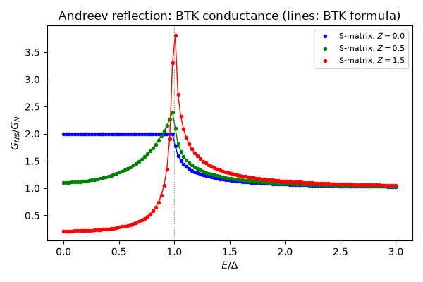
Z = 0.0: G_NS(0)/G_N = 2.000 (BTK 2.000)
Z = 0.5: G_NS(0)/G_N = 1.107 (BTK 1.111)
Z = 1.5: G_NS(0)/G_N = 0.213 (BTK 0.215)