Visualizing a Model: tbkit.plot.Plot

Every other example in this gallery reaches straight for matplotlib to plot a spectrum or a band structure by hand. tbkit.plot.Plot instead wraps the handful of plots that come up for any real-space model, directly from a System instance: the lattice itself (with or without its hoppings drawn on), the spectrum (optionally colored by sublattice polarization), the density of states, and an eigenstate’s spatial intensity.

import numpy as np

from tbkit.graphene import GrapheneLattice
from tbkit.system import System
from tbkit.plot import Plot
from tbkit.dos import density_of_states

A small graphene flake

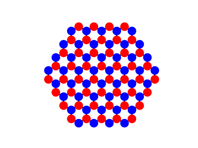
A zigzag hexagonal flake, small enough that the lattice and hopping plots below stay legible.

glat = GrapheneLattice()
glat.hexagon_zigzag(n=4)
sys = System(glat)
sys.set_onsite({'a': 0., 'b': 0.})
sys.set_hopping([{'n': 1, 't': 1.}])
sys.get_ham()
sys.get_eig(eigenvec=True)
plot = Plot(sys)
print('Flake: {} sites.'.format(glat.sites))

# Sanity check that holds for any bipartite lattice, field or not (see
# also the magnetic-field examples): the spectrum is exactly symmetric
# under E -> -E.
en = np.sort(sys.en.real)
assert np.allclose(en, -en[::-1], atol=1e-8)
print('Particle-hole symmetry E -> -E: exact to machine precision.')

Flake: 96 sites.
Particle-hole symmetry E -> -E: exact to machine precision.

The lattice, with hoppings drawn on

fig1 = plot.lattice(plt_hop=True)

Spectrum and sublattice polarization

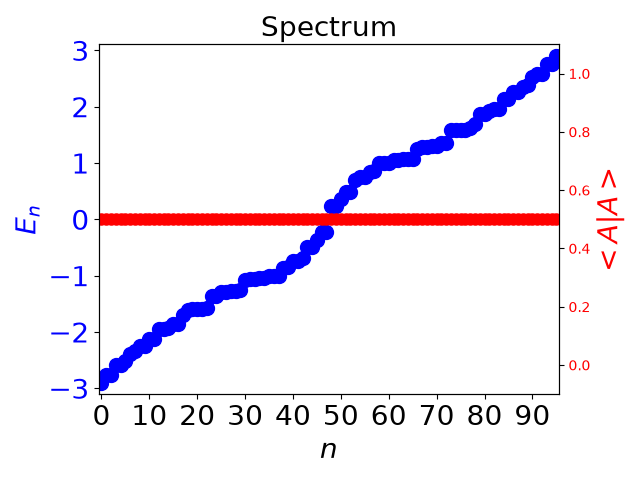
tag_pola='a' colors each eigenstate by how much of its weight sits on sublattice a – 1 for a state fully on a, 0 for fully on b. Every state’s a + b weight sums to exactly 1 (a normalized eigenvector split across the two sublattices), regardless of how it is distributed between them.

fig2 = plot.spectrum(tag_pola='a')
pola_sum = sys.pola.sum(axis=1)
print('Sublattice weights sum to 1 for every state: {} (min={:.6f}, max={:.6f}).'
           .format(np.allclose(pola_sum, 1.), pola_sum.min(), pola_sum.max()))
assert np.allclose(pola_sum, 1.)

Sublattice weights sum to 1 for every state: True (min=1.000000, max=1.000000).

Density of states

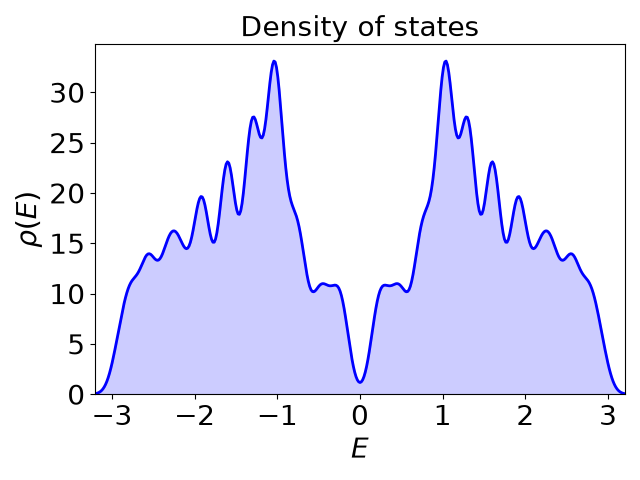
fig3 = plot.dos(broadening=0.1)
# The broadened DOS integrates back to the total number of states,
# regardless of the broadening kernel's width.
e_grid, rho = density_of_states(sys.en, broadening=0.1)
integral = np.trapezoid(rho, e_grid)
print('DOS integrates to {:.3f} states (flake has {}).'.format(integral, glat.sites))
assert abs(integral - glat.sites) < 0.5

DOS integrates to 95.997 states (flake has 96).

An eigenstate’s spatial intensity

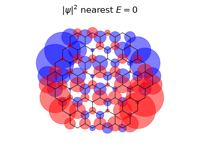
intensity_area() draws \(|\psi_i|^2\) as a disk at each site, sized by the local weight – here, for the state closest to zero energy.

i0 = np.argmin(np.abs(sys.en.real))
print('State closest to E=0: E={:.4f} (index {}).'.format(sys.en.real[i0], i0))
fig4 = plot.intensity_area(sys.intensity[:, i0], plt_hop=True,
                                              title=r'$|\psi|^2$ nearest $E=0$')

State closest to E=0: E=0.2294 (index 48).