Graphene: Real-Space Flake and Reciprocal-Space Bands

A from-scratch walkthrough of tbkit’s two complementary ways of looking at a Tight-Binding model:

• tbkit.lattice / tbkit.system – build a finite flake in real space and diagonalize it directly.

• tbkit.kspace – build the Bloch Hamiltonian \(H(\mathbf{k})\) of the infinite periodic lattice and compute a band structure along a k-path.

Graphene’s honeycomb lattice is the running example throughout tbkit’s History – its two bands touch linearly at the Brillouin zone corners, the massless-Dirac-fermion dispersion P. R. Wallace predicted in 1947, fifty-seven years before the material itself was isolated.

import numpy as np
import matplotlib.pyplot as plt

from tbkit.lattice import Lattice
from tbkit.system import System
from tbkit.plot import Plot
from tbkit.kspace import KSpace, reciprocal_vectors

Shared lattice geometry

A two-atom hexagonal unit cell (sublattices a, b) with a single nearest-neighbor hopping t.

DX, DY = 0.5 * 3 ** 0.5, 0.5
unit_cell = [{'tag': 'a', 'r0': (0., 0.)}, {'tag': 'b', 'r0': (DX, DY)}]
prim_vec = [(2 * DX, 0.), (DX, 1.5)]
t = 1.

Real space: a finite flake, diagonalized directly

get_lattice() tiles the unit cell into an 8x8-cell flake; System then builds and diagonalizes its real-space Hamiltonian.

# The honeycomb lattice this builds: two orbitals ('a' and 'b', drawn in
# different colours) per unit cell, each with three nearest neighbors on
# the other sublattice.
lat_small = Lattice(unit_cell=unit_cell, prim_vec=prim_vec)
lat_small.get_lattice(n1=5, n2=4)
vis = System(lat_small)
vis.set_hopping([{'n': 1, 't': t}])
fig_lat = Plot(vis).lattice(plt_hop=True, ms=12, figsize=(5.5, 4.5))

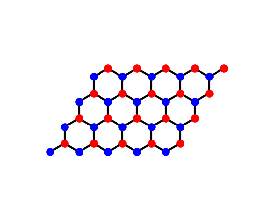
The flake actually diagonalized:

lat = Lattice(unit_cell=unit_cell, prim_vec=prim_vec)
lat.get_lattice(n1=8, n2=8)

sys = System(lat)
sys.set_hopping([{'n': 1, 't': t}])
sys.set_onsite({'a': 0., 'b': 0.})
sys.get_ham()
sys.get_eig()

fig, ax = plt.subplots()
ax.plot(sys.en.real, 'o')
ax.set_xlabel('state index $n$')
ax.set_ylabel('$E_n$')
ax.set_title('Graphene flake: real-space spectrum')
print('Real-space flake: {} sites.'.format(sys.lat.sites))

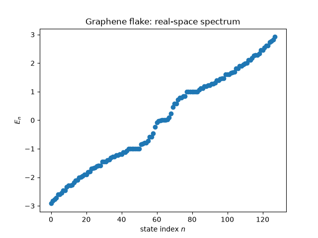
Real-space flake: 128 sites.

Reciprocal space: the Bloch Hamiltonian H(k) and its band structure

KSpace Bloch-sums the same nearest-neighbor hopping into \(H(\mathbf{k})\), and k_path() / plot_bands() diagonalize it along a path through the high-symmetry points \(\Gamma\), K, M.

kag = KSpace(lat)
kag.set_hopping([{'i': 0, 'j': 1, 'R': (0, 0), 't': t},
                        {'i': 0, 'j': 1, 'R': (-1, 0), 't': t},
                        {'i': 0, 'j': 1, 'R': (0, -1), 't': t}])

b1, b2 = (np.array(v) for v in reciprocal_vectors(prim_vec))
Gamma = np.zeros(2)
K = (b1 - b2) / 3
M = b1 / 2

kag.k_path([Gamma, K, M, Gamma], nk=60)
fig2 = kag.plot_bands(node_labels=[r'$\Gamma$', 'K', 'M', r'$\Gamma$'])

# Sanity check: the two bands must touch exactly at the Dirac point K.
en_K = np.linalg.eigvalsh(kag.get_ham(K))
print('Energies at K: {} (should be ~0, ~0 -- the Dirac point)'.format(en_K))

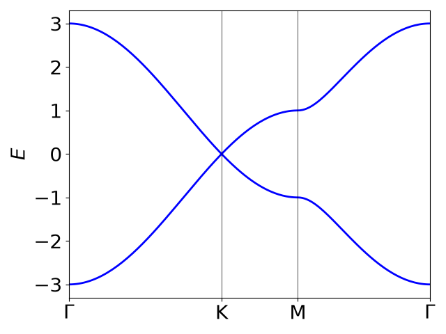
Energies at K: [-1.11022302e-16  1.11022302e-16] (should be ~0, ~0 -- the Dirac point)

Wallace’s 1947 linear dispersion near K

The historically defining result: near K the dispersion isn’t just gapless, it is linear (massless Dirac fermions), \(E(\mathbf{K}+\mathbf{q}) \approx \pm\frac{3}{2}ta|\mathbf{q}|\), with \(a\) the nearest-neighbor distance. See History for the historical context.

a = 1.
for q in (0.001, 0.01, 0.05):
    en_q = np.linalg.eigvalsh(kag.get_ham(K + np.array([q, 0.])))
    predicted = 1.5 * t * a * q
    print('|q|={:.3f}: E(K+q)={:.6f}, Wallace linear estimate={:.6f}'
               .format(q, en_q[1], predicted))
    assert np.isclose(en_q[1], predicted, rtol=0.02)
print('Linear (Dirac) dispersion near K confirmed to within 2% for |q|<=0.05.')

|q|=0.001: E(K+q)=0.001500, Wallace linear estimate=0.001500
|q|=0.010: E(K+q)=0.015037, Wallace linear estimate=0.015000
|q|=0.050: E(K+q)=0.075914, Wallace linear estimate=0.075000
Linear (Dirac) dispersion near K confirmed to within 2% for |q|<=0.05.