Magic-Angle Twisted Bilayer Graphene: Flat Moiré Bands

Twist two graphene sheets by a small angle \(\theta\) and a moiré pattern appears, with a period \(a/(2\sin\frac\theta2)\) of a hundred lattice constants. R. Bistritzer and A. H. MacDonald (2011) showed that the interlayer tunnelling \(w\) slows the Dirac electrons down,

\[\frac{v^*}{v} = \frac{1-3\alpha^2}{1+6\alpha^2}\, ,\qquad \alpha = \frac{w}{\hbar v k_\theta}\, ,\quad k_\theta = 2|\mathbf{K}|\sin\frac\theta2\, ,\]

until, at the magic angle \(\alpha = 1/\sqrt3\) (about \(1.1°\)), the two bands at charge neutrality become almost flat. In 2018 Y. Cao, P. Jarillo-Herrero and co-workers found correlated insulators and superconductivity in exactly those flat bands.

tbkit.moire.twisted_bilayer() builds the commensurate moiré cell of the atomistic model (the Slater-Koster \(p_z\) hoppings of Moon and Koshino, pz_hopping(), within and between the layers).

Why not 1.05° directly? The commensurate cell at \(\theta = 1.05°\) (\(m = 31\)) holds 11908 orbitals: one dense Bloch matrix takes 2.3 GB, too much for a gallery script. The physics depends on \(\alpha\) only, so we (i) check \(v^*/v\) against Bistritzer-MacDonald at larger angles, where \(\alpha\) is small, and (ii) reach the magic value of \(\alpha\) at \(\theta = 6°\) (364 orbitals) by scaling the interlayer hoppings (interlayer_scale), the continuum-scaling argument of the Bistritzer-MacDonald model.

import numpy as np
import matplotlib.pyplot as plt
from scipy.optimize import brentq

from tbkit.moire import commensurate_angle, magic_angle_parameter, twisted_bilayer


def moire_k(tbl):
    '''Corner K of the moire Brillouin zone.'''
    b1, b2 = tbl.rec_vec_k
    c = b2 if b1 @ b2 > 0 else b1 + b2
    return np.linalg.solve(2 * np.array([b1, c]), np.array([b1 @ b1, c @ c]))


def central(tbl, ks):
    '''The four bands at charge neutrality (two valleys, two bands).'''
    n = tbl.norb // 2
    return np.linalg.eigvalsh(tbl._bloch_ham(ks @ tbl.k_basis.T))[:, n - 2:n + 2]


def dirac_velocity(tbl, dq=1e-2):
    k = moire_k(tbl)
    e0, e1 = central(tbl, np.array([k, k * (1 + dq)]))
    return np.mean(np.abs(e1 - e0.mean())) / (dq * np.linalg.norm(k))

The moiré lattice

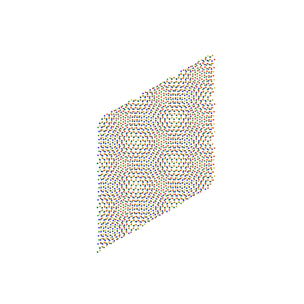
Two graphene layers twisted by \(\theta = 6.01°\) (\(m = 5\)), seen from above: layer 0 (sublattices ‘a’ and ‘b’, blue and red) and layer 1 (‘c’ and ‘d’, green and yellow), over \(3\times3\) moiré cells of 364 sites each (positions in nm). Where the layers’ sites coincide the stacking is locally AA; between those regions it is AB or BA. The pattern repeats with the moiré period, about 2.3 nm here.

moire_lat = twisted_bilayer(5).lat
assert len(moire_lat.unit_cell) == 364
assert abs(np.linalg.norm(moire_lat.prim_vec[0]) - 2.35) < 0.01
moire_lat.get_lattice(3, 3)
fig_lat = moire_lat.plot(ms=2, figsize=(6, 6))

Commensurate angles and the magic angle

\(m = 31\) gives \(\theta = 1.05°\). The Bistritzer-MacDonald tunnelling of the Moon-Koshino hoppings is \(w \approx 110\) meV, and \(v^* = 0\) at \(\theta \approx 1.1°\).

theta_31 = np.degrees(commensurate_angle(31))
w, _, _ = magic_angle_parameter(np.radians(1.05))
magic = brentq(lambda th: magic_angle_parameter(np.radians(th))[2], 0.8, 2.)
assert abs(theta_31 - 1.05) < 0.01 and abs(w - 0.11) < 0.005 and abs(magic - 1.1) < 0.1
print('m = 31: theta = {:.3f} deg, {} orbitals'.format(theta_31, 4 * (3 * 31**2 + 3 * 31 + 1)))
print('w = {:.1f} meV, first magic angle {:.2f} deg'.format(1e3 * w, magic))

m = 31: theta = 1.050 deg, 11908 orbitals
w = 110.8 meV, first magic angle 1.12 deg

The Dirac velocity follows Bistritzer and MacDonald

The velocity at the moiré K point, relative to that of decoupled layers, against \((1-3\alpha^2)/(1+6\alpha^2)\) for the same model.

rows = []
for m in (3, 5, 7):
    tbl = twisted_bilayer(m)
    v0 = dirac_velocity(twisted_bilayer(m, interlayer_scale=1e-9))
    ratio_tb = dirac_velocity(tbl) / v0
    _, alpha, ratio_bm = magic_angle_parameter(tbl.theta, t=-v0 / (1.5 * 0.142))
    assert abs(ratio_tb - ratio_bm) < 0.03
    rows.append((np.degrees(tbl.theta), alpha, ratio_tb, ratio_bm))
    print('theta = {:5.2f} deg  alpha = {:.3f}  v*/v: TB {:.3f}  BM {:.3f}'.format(*rows[-1]))

theta =  9.43 deg  alpha = 0.076  v*/v: TB 0.947  BM 0.950
theta =  6.01 deg  alpha = 0.119  v*/v: TB 0.877  BM 0.883
theta =  4.41 deg  alpha = 0.162  v*/v: TB 0.782  BM 0.796

Flat bands at the magic value of alpha

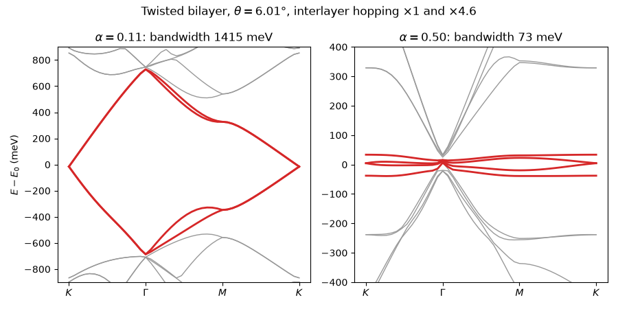
At \(\theta = 6.01°\) (\(m = 5\)), the interlayer hoppings scaled by 4.6 bring \(\alpha\) to 0.50, near the magic value of the lattice model: the bandwidth of the four central bands drops by more than an order of magnitude.

fig, axes = plt.subplots(1, 2, figsize=(9, 4.5), sharey=False)
widths = []
for ax, s, lim in zip(axes, (1., 4.6), (900, 400)):
    tbl = twisted_bilayer(5, interlayer_scale=s)
    k = moire_k(tbl)
    m_pt = tbl.rec_vec_k[0] / 2
    nodes = [k, 0 * k, m_pt, k]
    ks = np.concatenate([np.linspace(nodes[i], nodes[i + 1], 15, endpoint=False) for i in range(3)]
                                   + [nodes[-1:]])
    en = np.linalg.eigvalsh(tbl._bloch_ham(ks @ tbl.k_basis.T))
    n = tbl.norb // 2
    mid = en[:, n - 2:n + 2]
    widths.append(mid.max() - mid.min())
    e0 = mid.mean()
    x = np.arange(len(ks))
    ax.plot(x, 1e3 * (en[:, n - 8:n + 8] - e0), c='0.6', lw=1)
    ax.plot(x, 1e3 * (mid - e0), c='C3', lw=2)
    _, alpha, _ = magic_angle_parameter(tbl.theta, interlayer_scale=s)
    assert s == 1. or abs(alpha - 0.50) < 0.01
    ax.set_title(r'$\alpha = {:.2f}$: bandwidth {:.0f} meV'.format(alpha, 1e3 * widths[-1]))
    ax.set_xticks([0, 15, 30, 45])
    ax.set_xticklabels([r'$K$', r'$\Gamma$', r'$M$', r'$K$'])
    ax.set_ylim(-lim, lim)
axes[0].set_ylabel('$E - E_0$ (meV)')
assert widths[0] / widths[1] > 15
print('bandwidth: {:.0f} meV -> {:.0f} meV'.format(1e3 * widths[0], 1e3 * widths[1]))
fig.suptitle(r'Twisted bilayer, $\theta = 6.01°$, interlayer hopping $\times 1$ and $\times 4.6$')
fig.tight_layout()

bandwidth: 1415 meV -> 73 meV