From Real Space to k-Space and Back: the Haldane Model on a Torus

tbkit has two pipelines: System diagonalizes a finite lattice in real space, KSpace the Bloch Hamiltonian \(H(\mathbf{k})\) of the infinite one. tbkit.bridges moves a model between them:

• kspace_from_system() reads the Bloch model off a translation-invariant System built the real-space way;

• finite_system() (and finite_model(), its sparse Hamiltonian with the site positions) cuts a finite sample – open, or a torus – out of a KSpace model.

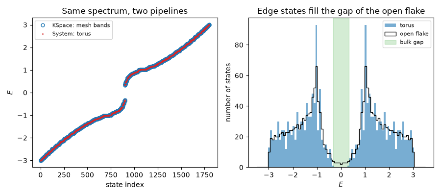
The proof that both describe the same model: on an \(N_1\times N_2\) torus the real-space spectrum is exactly the set of Bloch energies on the \(N_1\times N_2\) Brillouin-zone mesh. The running example is F. D. M. Haldane’s Chern insulator, set up with the real-space selectors (neighbour order, angle, sublattice pair) in both pipelines.

import numpy as np
import matplotlib.pyplot as plt

from tbkit import lattices
from tbkit.system import System
from tbkit.kspace import KSpace
from tbkit.bridges import kspace_from_system, finite_system, finite_model
from tbkit.plot import Plot

The Haldane model, by neighbour order

Nearest neighbours \(t_1\); second neighbours \(t_2e^{i\phi}\) on sublattice a along the three directions at 0, 120 and 240 degrees (\(t_2e^{-i\phi}\) against them), the opposite on sublattice b. The stored bond at 60 degrees is the one at 240 degrees reversed, hence the conjugate. The ‘aa’ and ‘bb’ bonds are addressed by 'tag' and 'ang', exactly as in System.set_hopping. A staggered potential \(\pm M\) completes the model.

t1, t2, phi, M = 1., 0.1, np.pi / 2, 0.2
p, q = t2 * np.exp(1j * phi), t2 * np.exp(-1j * phi)
list_hop = [{'n': 1, 't': t1},
                  {'n': 2, 'tag': 'aa', 'ang': 0., 't': p}, {'n': 2, 'tag': 'aa', 'ang': 60., 't': q},
                  {'n': 2, 'tag': 'aa', 'ang': 120., 't': p},
                  {'n': 2, 'tag': 'bb', 'ang': 0., 't': q}, {'n': 2, 'tag': 'bb', 'ang': 60., 't': p},
                  {'n': 2, 'tag': 'bb', 'ang': 120., 't': q}]
onsite = {'a': M, 'b': -M}

hal = KSpace(lattices.honeycomb())
hal.set_hopping(list_hop)
hal.set_onsite(onsite)

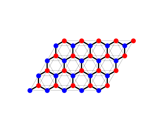
The model on a patch of \(5\times4\) cells (finite_system()), bond widths proportional to the amplitudes: sublattices a and b in two colours, the nearest-neighbour bonds \(t_1\) (thick) and the second-neighbour ones \(t_2\) (thin).

fig_lat = Plot(finite_system(hal, (5, 4))).lattice(plt_hop=True, ms=12, figsize=(5.5, 4.5))

Real space to k-space

The same list, given to a finite System (a flake, open boundaries): kspace_from_system() recovers the Bloch Hamiltonian from its matrix elements, cell by cell.

lat = lattices.honeycomb()
lat.get_lattice(8, 8)
flake = System(lat)
flake.set_hopping(list_hop)
flake.set_onsite(onsite)
from_flake = kspace_from_system(flake)
for k in np.random.default_rng(1).uniform(-4., 4., (20, 2)):
    assert np.allclose(from_flake.get_ham(k), hal.get_ham(k), atol=1e-14)
# ... and it is the textbook Haldane model: |Chern number| = 1 at M < 3 sqrt(3) t2
chern = hal.chern_number(bands=[0], nk=30)
print('Chern number of the lower band: {:.6f}'.format(chern))
assert abs(abs(chern) - 1) < 1e-9

Chern number of the lower band: -1.000000

k-space to real space: a torus

finite_system() builds a System on a \(30\times 30\) torus (1800 sites). Its spectrum equals the Bloch bands on the \(30\times 30\) mesh, which contains the Dirac points K and K’: there the gaps are \(2|M \mp 3\sqrt{3}t_2\sin\phi|\), and the smaller one is the band gap.

N = 30
torus = finite_system(hal, (N, N), periodic=True)
torus.get_ham()
torus.get_eig()
mesh = np.sort(hal.mesh_bands(N).ravel())
print('max |E_torus - E_mesh| = {:.2e}'.format(np.abs(torus.en - mesh).max()))
assert torus.lat.sites == 2 * N * N
assert np.allclose(torus.en, mesh, atol=1e-10)

half = N * N
gap_torus = torus.en[half] - torus.en[half - 1]
gap_K = 2 * abs(M - 3 * np.sqrt(3) * t2 * np.sin(phi))
print('torus gap = {:.6f}, 2|M - 3 sqrt(3) t2| = {:.6f}'.format(gap_torus, gap_K))
assert abs(gap_torus - gap_K) < 1e-10

max |E_torus - E_mesh| = 4.09e-14
torus gap = 0.639230, 2|M - 3 sqrt(3) t2| = 0.639230

The same sample with open boundaries is a Chern-insulator flake: chiral edge states fill the bulk gap, where the torus has no state at all.

open_flake = finite_system(hal, (N, N))
open_flake.get_ham()
open_flake.get_eig()
in_gap = np.abs(open_flake.en) < 0.5 * gap_K / 2
print('states inside the bulk gap: torus {}, open flake {}'.format(
      int(np.sum(np.abs(torus.en) < 0.5 * gap_K / 2)), int(in_gap.sum())))
assert not np.any(np.abs(torus.en) < gap_K / 2 - 1e-9)
assert in_gap.sum() > 10

# finite_model gives the sparse matrix and the site positions directly
ham, positions, tags = finite_model(hal, (N, N))
assert np.allclose(ham.toarray(), open_flake.ham.toarray(), atol=1e-14)
assert positions.shape == (2 * N * N, 2)

states inside the bulk gap: torus 0, open flake 12

Spectra

fig, (ax1, ax2) = plt.subplots(1, 2, figsize=(9, 4))
ax1.plot(mesh, 'o', ms=5, mfc='none', color='C0', label='KSpace: mesh bands')
ax1.plot(torus.en, '.', ms=2, color='C3', label='System: torus')
ax1.set_xlabel('state index')
ax1.set_ylabel('$E$')
ax1.set_title('Same spectrum, two pipelines')
ax1.legend(fontsize=8)
bins = np.linspace(-3.5, 3.5, 90)
ax2.hist(torus.en, bins=bins, alpha=0.6, label='torus')
ax2.hist(open_flake.en.real, bins=bins, histtype='step', color='k', label='open flake')
ax2.axvspan(-gap_K / 2, gap_K / 2, color='C2', alpha=0.2, label='bulk gap')
ax2.set_xlabel('$E$')
ax2.set_ylabel('number of states')
ax2.set_title('Edge states fill the gap of the open flake')
ax2.legend(fontsize=8)
fig.tight_layout()
plt.show()