Zak’s Magnetic Translation Group: the Magnetic Supercell at Rational Flux

A uniform magnetic field breaks the translation symmetry of a lattice’s Hamiltonian: the vector potential grows across the sample, so the Peierls phases of a bond and of its translate differ. Zak (1964) showed that a translation followed by a gauge transformation is still a symmetry – a magnetic translation – but two of them commute only up to the flux they enclose,

\[T_1 T_2 = e^{2\pi i\alpha}\, T_2 T_1\, ,\]

with \(\alpha\) the flux per unit cell in flux quanta. For a rational flux \(\alpha = p/q\), \(T_1^q\) and \(T_2\) commute again: a magnetic unit cell of \(q\) cells has Bloch states, the band splits into \(q\) subbands, and since \(T_1\) moves a Bloch state from \(k_2\) to \(k_2 + 2\pi p/q\), every level appears \(q\) times across the magnetic Brillouin zone.

magnetic_supercell() builds that magnetic unit cell for any 2D KSpace model, here the square lattice.

import numpy as np
import matplotlib.pyplot as plt

import tbkit.lattices as lattices
from tbkit.bridges import finite_system
from tbkit.kspace import magnetic_supercell
from tbkit.plot import Plot


square = [{'i': 0, 'j': 0, 'R': (1, 0), 't': 1.}, {'i': 0, 'j': 0, 'R': (0, 1), 't': 1.}]


def harper(p, q, k):
    r'''Harper's q x q matrix: the same model written by hand in the Landau gauge.'''
    onsite = np.diag(2 * np.cos(k[1] + 2 * np.pi * p / q * np.arange(q)))
    hop = np.eye(q, k=1, dtype=complex)
    hop[q - 1, 0] = np.exp(1j * k[0] * q)  # into the next magnetic cell (q >= 3)
    return onsite + hop + hop.conj().T

The lattice

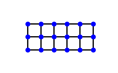
The square lattice, one site per cell and a nearest-neighbour hopping, here as six of its magnetic cells at flux \(1/3\) (magnetic_supercell(), then finite_system()): three sites along \(\mathbf{a}_1\) per magnetic cell. The Peierls phases change the hoppings’ phases, not their amplitudes, so every bond is drawn alike.

fig_lat = Plot(finite_system(magnetic_supercell(lattices.square(), square, 1, 3), (2, 3))).lattice(plt_hop=True, ms=12, figsize=(4, 2.5))

The magnetic unit cell is Harper’s equation

At flux \(p/q\) the magnetic cell holds \(q\) sites along \(\mathbf{a}_1\), and its Bloch Hamiltonian is Harper’s (1955) \(q \times q\) matrix: hopping along the cell, and the bonds along \(\mathbf{a}_2\) turned into an onsite \(2\cos(k_2 + 2\pi\alpha m)\) by the Peierls phase of row m.

rng = np.random.default_rng(0)
for p, q in [(1, 3), (2, 5), (3, 7)]:
    mag = magnetic_supercell(lattices.square(), square, p, q)
    assert len(mag.lat.unit_cell) == q
    for k in rng.uniform(-np.pi, np.pi, (4, 2)):
        k[0] /= q  # inside the magnetic Brillouin zone
        assert np.allclose(np.linalg.eigvalsh(mag.get_ham(k)),
                           np.linalg.eigvalsh(harper(p, q, k)), atol=1e-10)
print('magnetic_supercell matches Harper\'s matrix at 1/3, 2/5 and 3/7: OK')

magnetic_supercell matches Harper's matrix at 1/3, 2/5 and 3/7: OK

The q-fold degeneracy of the magnetic translations

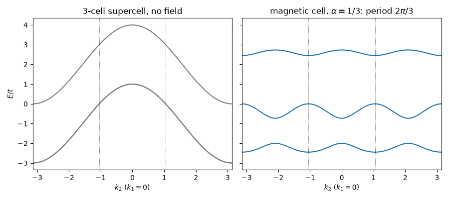
The magnetic Brillouin zone is \(2\pi/q\) wide along \(k_1\) but still \(2\pi\) along \(k_2\). A magnetic translation along \(\mathbf{a}_1\) shifts \(k_2\) by \(2\pi/q\) (times p), so the spectrum repeats \(q\) times along \(k_2\). Without the field, the same \(q\)-cell supercell (p=0) has no such symmetry: the degeneracy comes from the non-commuting translations, not from the larger cell.

p, q = 1, 3
mag = magnetic_supercell(lattices.square(), square, p, q)
plain = magnetic_supercell(lattices.square(), square, 0, q)
for k in rng.uniform(-np.pi, np.pi, (5, 2)):
    shift = np.array([0., 2 * np.pi / q])
    assert np.allclose(np.linalg.eigvalsh(mag.get_ham(k)), np.linalg.eigvalsh(mag.get_ham(k + shift)))
    assert not np.allclose(np.linalg.eigvalsh(plain.get_ham(k)), np.linalg.eigvalsh(plain.get_ham(k + shift)))
print('alpha = 1/3: E(k1, k2) = E(k1, k2 + 2 pi/3), absent at zero flux: OK')

k2 = np.linspace(-np.pi, np.pi, 301)
bands = np.array([np.linalg.eigvalsh(mag.get_ham([0., k])) for k in k2])
bands0 = np.array([np.linalg.eigvalsh(plain.get_ham([0., k])) for k in k2])

fig, axes = plt.subplots(1, 2, figsize=(9, 4), sharey=True)
axes[0].plot(k2, bands0, 'C7')
axes[0].set_title('3-cell supercell, no field')
axes[1].plot(k2, bands, 'C0')
axes[1].set_title(r'magnetic cell, $\alpha = 1/3$: period $2\pi/3$')
for ax in axes:
    for x in 2 * np.pi * np.arange(-1, 2) / q - np.pi / q:
        ax.axvline(x, c='k', lw=0.5, ls=':')
    ax.set_xlabel('$k_2$ ($k_1 = 0$)')
    ax.set_xlim(-np.pi, np.pi)
axes[0].set_ylabel('$E/t$')
fig.tight_layout()

alpha = 1/3: E(k1, k2) = E(k1, k2 + 2 pi/3), absent at zero flux: OK

q subbands at every rational flux

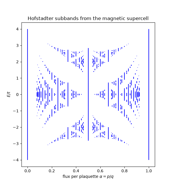
On a mesh of the magnetic Brillouin zone, the band at \(p/q\) breaks into exactly \(q\) subbands, separated by gaps for odd \(q\) (for even \(q\) the two central ones touch at \(E = 0\)). Plotting their ranges over all \(p/q\) with \(q \le 13\) draws Hofstadter’s butterfly from bulk Bloch bands alone, with none of the edge states that fill the gaps of a finite flake.

fluxes = sorted({(int(p // np.gcd(p, q)), int(q // np.gcd(p, q))) for q in range(1, 14) for p in range(q + 1)},
                key=lambda pq: pq[0] / pq[1])
fig2, ax = plt.subplots(figsize=(6, 6.5))
for p, q in fluxes:
    mb = magnetic_supercell(lattices.square(), square, p, q).mesh_bands(12)
    assert mb.shape[1] == q
    lo, hi = mb.min(axis=0), mb.max(axis=0)
    if q % 2:
        assert np.all(lo[1:] > hi[:-1])  # q separated subbands
    ax.vlines(np.full(q, p / q), lo, hi, color='b', lw=1.5)
print('q subbands at all {} fluxes p/q, q <= 13, separated for odd q: OK'.format(len(fluxes)))
ax.set_xlabel(r'flux per plaquette $\alpha = p/q$')
ax.set_ylabel('$E/t$')
ax.set_title('Hofstadter subbands from the magnetic supercell')

q subbands at all 59 fluxes p/q, q <= 13, separated for odd q: OK

Text(0.5, 1.0, 'Hofstadter subbands from the magnetic supercell')