The Hubbard Model: Magnetism of Graphene’s Zigzag Edges

J. Hubbard (1963) – together with Gutzwiller and Kanamori, the same year – reduced the problem of interacting electrons in narrow bands to its bare bones: hopping between neighbouring sites, and a repulsion \(U\) between two electrons on the same site,

\[H = \sum_{\langle ij\rangle\sigma} t\,c^\dagger_{i\sigma}c_{j\sigma} + U\sum_i n_{i\uparrow}n_{i\downarrow}\, .\]

It remains the reference model of magnetism, Mott insulators and (doped) high-temperature superconductivity.

In the unrestricted Hartree-Fock approximation (hubbard_mean_field()), each spin moves in the average density of the other. On a graphene flake, the zigzag edges carry nearly flat bands of states at \(E = 0\); the repulsion splits them, magnetizing each edge ferromagnetically, and neighbouring edges – which end on opposite sublattices – in opposite directions (Fujita et al. 1996; Son, Cohen and Louie 2006). The flake as a whole stays a singlet, \(S_z = 0\), as Lieb’s theorem requires for equal sublattices.

import numpy as np
import matplotlib.pyplot as plt

from tbkit.graphene import GrapheneLattice
from tbkit.meanfield import hubbard_mean_field
from tbkit.plot import Plot
from tbkit.system import System

t = -1.


def flake(n):
    lat = GrapheneLattice()
    lat.hexagon_zigzag(n=n)
    sys = System(lat)
    sys.set_hopping([{'n': 1, 't': t}])
    sys.get_ham()
    neighbours = np.bincount(np.concatenate([sys.hop['i'], sys.hop['j']]).astype(int), minlength=lat.sites)
    return lat, sys, neighbours == 2  # the outermost atoms of the zigzag edges


def solve(sys, U):
    # start from a small staggered magnetization (a symmetric start has no
    # reason to magnetize at all)
    up = np.where(sys.lat.coor['tag'] == 'a', 0.55, 0.45)
    return hubbard_mean_field(sys.ham, U, sys.lat.sites, n_up=up, n_dn=1 - up)

The flake

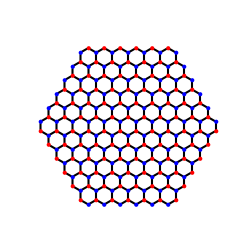
A hexagonal graphene flake with six zigzag edges. The two sublattices (‘a’ and ‘b’) are drawn in different colours: each edge ends on one of them, alternating from edge to edge.

lat, sys, edge = flake(6)
fig_lat = Plot(sys).lattice(plt_hop=True, ms=6, figsize=(5, 5))

Edge moments, opposite on opposite sublattices

A = lat.coor['tag'] == 'a'
res = solve(sys, 2.)
m = res.magnetization
print('{} sites; U = 2|t|: S_z = {:.1e}; edge moments {:.3f} (A) and {:.3f} (B); bulk |m| {:.3f}.'
          .format(lat.sites, res.total_spin, m[edge & A].mean(), m[edge & ~A].mean(), np.abs(m[~edge]).mean()))
assert abs(res.total_spin) < 1e-8
assert np.all(m[edge & A] > 0) and np.all(m[edge & ~A] < 0)
assert np.abs(m[edge]).mean() > 2 * np.abs(m[~edge]).mean()

fig, ax = plt.subplots(figsize=(5.5, 5))
sc = ax.scatter(lat.coor['x'], lat.coor['y'], c=m, cmap='RdBu', vmin=-0.2, vmax=0.2, s=40)
fig.colorbar(sc, ax=ax, label=r'$m_i = (n_{i\uparrow} - n_{i\downarrow})/2$')
ax.set_aspect('equal')
ax.axis('off')
ax.set_title('Hubbard mean field, $U = 2|t|$: magnetic zigzag edges')

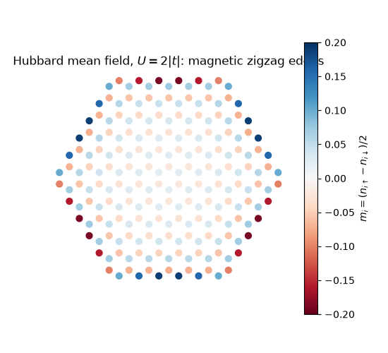
216 sites; U = 2|t|: S_z = -4.2e-15; edge moments 0.150 (A) and -0.150 (B); bulk |m| 0.044.

Text(0.5, 1.0, 'Hubbard mean field, $U = 2|t|$: magnetic zigzag edges')

A threshold that closes as the edges grow

In a finite flake the edge states hybridize across the corners and are split by a small gap: they magnetize only once \(U\) beats it. That threshold shrinks as the edges get longer (and vanishes for an infinite zigzag edge, whose band is exactly flat).

for n, U in ((4, 1.5), (6, 1.5)):
    lat_n, sys_n, edge_n = flake(n)
    moment = np.abs(solve(sys_n, U).magnetization[edge_n]).mean()
    print('{} sites, U = {}|t|: mean edge moment {:.3f}'.format(lat_n.sites, U, moment))
    assert (moment > 0.05) if n == 6 else (moment < 1e-6)

96 sites, U = 1.5|t|: mean edge moment 0.000
216 sites, U = 1.5|t|: mean edge moment 0.074