k·p Theory on a Lattice: from a Continuum Hamiltonian to Tight-Binding

The k·p method of J. M. Luttinger and W. Kohn (1955) and E. O. Kane (1957) describes the electrons of a semiconductor near a band edge by a small matrix that is a polynomial in the crystal momentum \(\mathbf{k}\). The effective mass \(k^2/2m^*\) is its simplest case. The Bernevig-Hughes-Zhang (BHZ) model of HgTe quantum wells is a two-band one. Devices and topology are computed on lattices, so the continuum model is discretized: \(k_x = -i\partial_x\) becomes a finite difference on a square grid of spacing \(a\).

discretize() does it for any sympy expression or string in k_x, k_y, k_z and returns a KSpace. This example checks the stencils, the \(O(a^2)\) convergence to the continuum bands, and that the lattice model carries the topology of the inverted BHZ band structure into a real-space flake.

import numpy as np
import matplotlib.pyplot as plt
import sympy

from tbkit.bridges import finite_system
from tbkit.continuum import discretize, discretize_symbolic
from tbkit.plot import Plot

The effective mass: a nearest-neighbour chain

\(k_x^2/2m^*\) becomes \(-(\psi_{n+1} - 2\psi_n + \psi_{n-1})/2m^*a^2\): a hopping \(-1/2m^*a^2\) and an onsite energy \(1/m^*a^2\), whose band \((1 - \cos ka)/m^*a^2\) is \(k^2/2m^*\) up to \(O(k^4a^2)\). discretize_symbolic() shows the hoppings before any number is put in.

hops = discretize_symbolic('k_x**2 / (2*m)')
for R, T in hops.items():
    print('T{} = {}'.format(R, T[0, 0]))
a_, m_ = sympy.symbols('a m')
assert sympy.simplify(hops[(1,)][0, 0] + 1 / (2 * m_ * a_**2)) == 0
assert sympy.simplify(hops[(0,)][0, 0] - 1 / (m_ * a_**2)) == 0

T(-1,) = -1/(2*a**2*m)
T(0,) = 1/(a**2*m)
T(1,) = -1/(2*a**2*m)

The BHZ model, discretized

One spin block of the BHZ Hamiltonian,

\[H(\mathbf{k}) = A(k_x\sigma_x - k_y\sigma_y) + (M - Bk^2)\sigma_z,\]

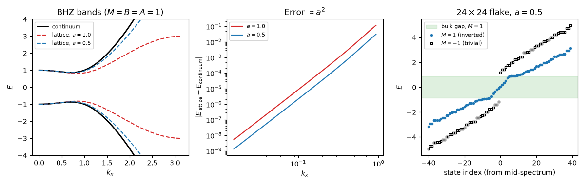
with the free symbols \(A, B, M\) left as parameters of the lattice model: they are set by get_ham(k, M=...) or set_params, without discretizing again. The lattice bands follow the continuum ones near \(\Gamma\), with an error that falls as \(a^2\). Far from \(\Gamma\) the lattice band bends back to the zone boundary \(\pi/a\), where the continuum one keeps growing.

BHZ = 'A*(k_x*sigma_x - k_y*sigma_y) + (M - B*(k_x**2 + k_y**2))*sigma_z'
params = {'A': 1., 'B': 1., 'M': 1.}


def continuum_bands(k, A, B, M):
    d = np.sqrt((A * k)**2 + (M - B * k**2)**2)
    return np.stack([-d, d], axis=1)


kx = np.linspace(0., np.pi, 200)
models = {a: discretize(BHZ, a=a) for a in (1., 0.5)}
bands = {a: np.array([np.linalg.eigvalsh(ks.get_ham((k, 0.), **params)) for k in kx])
         for a, ks in models.items()}
exact = continuum_bands(kx, **params)
small = kx <= 0.3
errors = {a: np.abs(bands[a][small] - exact[small]).max() for a in bands}
print('max band error for k <= 0.3: a = 1: {:.2e}, a = 0.5: {:.2e}, ratio {:.2f}'.format(
      errors[1.], errors[0.5], errors[1.] / errors[0.5]))
assert np.allclose(bands[1.][0], exact[0], atol=1e-12)   # exact at Gamma
assert 3.8 < errors[1.] / errors[0.5] < 4.2               # O(a^2)

max band error for k <= 0.3: a = 1: 7.53e-04, a = 0.5: 1.91e-04, ratio 3.94

Band inversion and the Chern number

The continuum model is topological when \(M/B > 0\) (the bands are inverted at \(\Gamma\)), but its Chern number is only defined up to the behaviour at \(k\to\infty\). The lattice closes the Brillouin zone and gives an integer: \(|C| = 1\) for \(M/B > 0\) and 0 for \(M/B < 0\), as long as \(M/B\) stays below \(4/a^2\), where the lattice closes the gap again at \(X = (\pi/a, 0)\). The sweep only changes the parameter.

bhz = models[0.5]
masses = np.linspace(-2., 2., 9)
cherns = []
for M in masses:
    bhz.set_params(A=1., B=1., M=float(M))
    cherns.append(bhz.chern_number(bands=[0], nk=40) if M != 0 else np.nan)
cherns = np.array(cherns)
print('Chern numbers vs M:', np.round(cherns, 6))
assert np.allclose(np.abs(cherns[masses > 0]), 1., atol=1e-6)
assert np.allclose(cherns[masses < 0], 0., atol=1e-6)
gap_X = np.ptp(np.linalg.eigvalsh(bhz.get_ham((2 * np.pi, 0.), A=1., B=1., M=4 / 0.5**2)))
assert gap_X < 1e-12

Chern numbers vs M: [ 0. -0.  0.  0. nan -1. -1. -1. -1.]

Edge states of a real-space flake

finite_system() cuts a \(24\times 24\) flake out of the lattice model (open boundaries). In the inverted regime, edge states fill the bulk gap \(|E| < \Delta/2\) (their level spacing, about \(2\pi A\) over the perimeter, sets how many). In the trivial one, nothing does.

spectra, gaps = {}, {}
for M in (1., -1.):
    bhz.set_params(A=1., B=1., M=M)
    gaps[M] = np.diff(bhz.mesh_bands((40, 40)), axis=1).min()
    flake = finite_system(bhz, (24, 24))
    flake.get_ham()
    flake.get_eig()
    spectra[M] = flake.en.real
in_gap = {M: int(np.sum(np.abs(spectra[M]) < gaps[M] / 2)) for M in spectra}
print('bulk gaps: {}, flake states with |E| < gap/2: {}'.format(
      {M: round(g, 3) for M, g in gaps.items()}, in_gap))
assert in_gap[1.] >= 8 and in_gap[-1.] == 0

bulk gaps: {1.0: np.float64(1.72), -1.0: np.float64(2.0)}, flake states with |E| < gap/2: {1.0: 10, -1.0: 0}

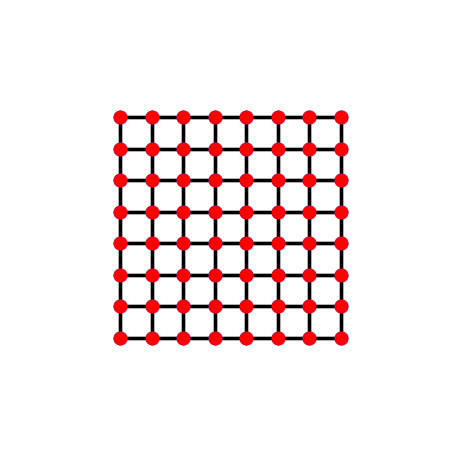
The lattice of the flake, here \(8\times8\) cells of it: a square grid, each site holding the two orbitals of the spin block (drawn on top of each other), joined by the nearest-neighbour hoppings of the discretized model.

fig_flake = Plot(finite_system(bhz, (8, 8))).lattice(plt_hop=True, ms=10, c=0.6, figsize=(4.5, 4.5))

Bands, convergence and edge states

fig, (ax1, ax2, ax3) = plt.subplots(1, 3, figsize=(12, 3.8))
ax1.plot(kx, exact, 'k-', lw=2, label=['continuum', None])
for a, c in zip(bands, ('C3', 'C0')):
    ax1.plot(kx, bands[a], '--', color=c, label=['lattice, $a={}$'.format(a), None])
ax1.set_ylim(-4, 4)
ax1.set_xlabel('$k_x$')
ax1.set_ylabel('$E$')
ax1.set_title('BHZ bands ($M=B=A=1$)')
ax1.legend(fontsize=8)
ks_err = kx[1:60]
for a, c in zip(bands, ('C3', 'C0')):
    ax2.loglog(ks_err, np.abs(bands[a][1:60, 1] - exact[1:60, 1]), color=c,
               label='$a={}$'.format(a))
ax2.set_xlabel('$k_x$')
ax2.set_ylabel(r'$|E_{\rm lattice} - E_{\rm continuum}|$')
ax2.set_title(r'Error $\propto a^2$')
ax2.legend(fontsize=8)
half = len(spectra[1.]) // 2
idx = np.arange(-40, 40)
ax3.axhspan(-gaps[1.] / 2, gaps[1.] / 2, color='C2', alpha=0.15, label='bulk gap, $M=1$')
ax3.plot(idx, np.sort(spectra[1.])[half + idx], 'o', ms=3, color='C0', label='$M=1$ (inverted)')
ax3.plot(idx, np.sort(spectra[-1.])[half + idx], 's', ms=3, mfc='none', color='k',
         label='$M=-1$ (trivial)')
ax3.set_xlabel('state index (from mid-spectrum)')
ax3.set_ylabel('$E$')
ax3.set_title(r'$24\times 24$ flake, $a=0.5$')
ax3.legend(fontsize=8)
fig.tight_layout()
plt.show()