Flat-Band Lattices: Kagome and Lieb

Some lattice geometries host a perfectly flat (dispersionless) band with uniform nearest-neighbor hopping alone – destructive interference confines an eigenstate to a small loop of sites (a single hexagon on kagome, a single “plus sign” of four sites on Lieb) with exactly zero amplitude everywhere else, for every Bloch momentum simultaneously. A flat band’s macroscopic degeneracy is the natural home for strong-correlation physics: Lieb’s theorem guarantees the half-filled Hubbard model on a bipartite lattice with an unequal number of sites per sublattice (as Lieb’s own lattice has, 2 vs 1) is a ferromagnet, for any nonzero repulsion U – one of the very few rigorous, non-perturbative results in the many-body problem. tbkit.lattices provides both lattices ready-made.

import numpy as np
import matplotlib.pyplot as plt

import tbkit.lattices as lattices
from tbkit.system import System
from tbkit.plot import Plot
from tbkit.kspace import KSpace, reciprocal_vectors


def kagome_kspace(t=1.):
    lat = lattices.kagome()
    kag = KSpace(lat)
    kag.set_hopping([{'i': 0, 'j': 1, 'R': (0, 0), 't': t},
                            {'i': 0, 'j': 1, 'R': (-1, 0), 't': t},
                            {'i': 0, 'j': 2, 'R': (0, 0), 't': t},
                            {'i': 0, 'j': 2, 'R': (0, -1), 't': t},
                            {'i': 1, 'j': 2, 'R': (0, 0), 't': t},
                            {'i': 1, 'j': 2, 'R': (1, -1), 't': t}])
    return kag, lat


def lieb_kspace(t=1.):
    lat = lattices.lieb()
    lb = KSpace(lat)
    lb.set_hopping([{'i': 0, 'j': 1, 'R': (0, 0), 't': t},
                          {'i': 0, 'j': 1, 'R': (-1, 0), 't': t},
                          {'i': 0, 'j': 2, 'R': (0, 0), 't': t},
                          {'i': 0, 'j': 2, 'R': (0, -1), 't': t}])
    return lb, lat

The two lattices

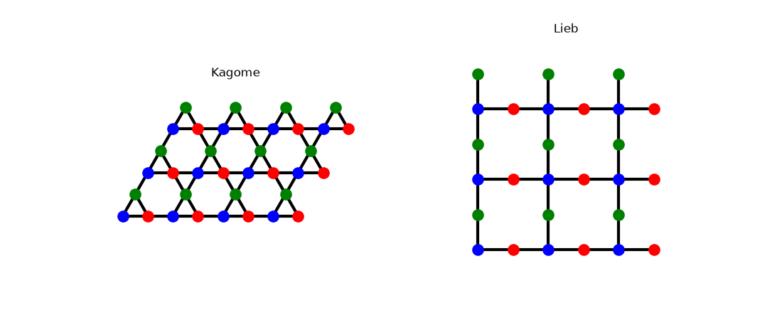
Both flat bands come from the geometry: a unit cell with more sites than there are independent ways for an electron to leave it, so some combination of orbitals interferes destructively and cannot disperse. The kagome lattice is corner-sharing triangles (three sites per cell, one per colour); the Lieb lattice is a square lattice with an extra site on every bond.

def draw_lattice(build_lat, n1, n2, ax):
    '''Draw a finite patch of the lattice, with its nearest-neighbor bonds.'''
    patch = build_lat()
    patch.get_lattice(n1=n1, n2=n2)
    vis = System(patch)
    vis.set_hopping([{'n': 1, 't': 1.}])
    Plot(vis).lattice(plt_hop=True, ms=12, ax=ax)


fig_lat, axes_lat = plt.subplots(1, 2, figsize=(11, 4.5))
draw_lattice(lattices.kagome, n1=4, n2=3, ax=axes_lat[0])
axes_lat[0].set_title('Kagome')
draw_lattice(lattices.lieb, n1=3, n2=3, ax=axes_lat[1])
axes_lat[1].set_title('Lieb')

Text(0.5, 1.0, 'Lieb')

Band structures and flatness check

Both lattices’ bands are computed along \(\Gamma \to X \to M \to \Gamma\), and the flat band’s bandwidth is checked to be numerically zero.

t = 1.
fig, axes = plt.subplots(1, 2, figsize=(10, 4.5))

for ax, (build, name, flat_energy, node_pts) in zip(axes, [
    (kagome_kspace, 'Kagome', -2*t, None),
    (lieb_kspace, 'Lieb', 0., None),
]):
    ks_obj, lat = build(t)
    b1, b2 = (np.array(v) for v in reciprocal_vectors(lat.prim_vec))
    Gamma, X, M = np.zeros(2), b1/2, (b1 + b2)/2
    ks_obj.k_path([Gamma, X, M, Gamma], nk=80)
    for n in range(ks_obj.norb):
        ax.plot(ks_obj.ks_dist, ks_obj.en[:, n], 'b', lw=1.5)
    ax.axhline(flat_energy, color='r', ls='--', lw=1, alpha=0.7)
    ax.set_xticks(ks_obj.nodes)
    ax.set_xticklabels([r'$\Gamma$', 'X', 'M', r'$\Gamma$'])
    ax.set_title('{} lattice (flat band at E={})'.format(name, flat_energy))
    ax.set_ylabel('$E$')

    flat_band = ks_obj.en[:, 0 if name == 'Kagome' else 1]
    flat_band_flatness = flat_band.max() - flat_band.min()
    print('{}: flat band bandwidth = {:.2e} (should be ~0)'.format(name, flat_band_flatness))
    assert flat_band_flatness < 1e-8

fig.tight_layout()

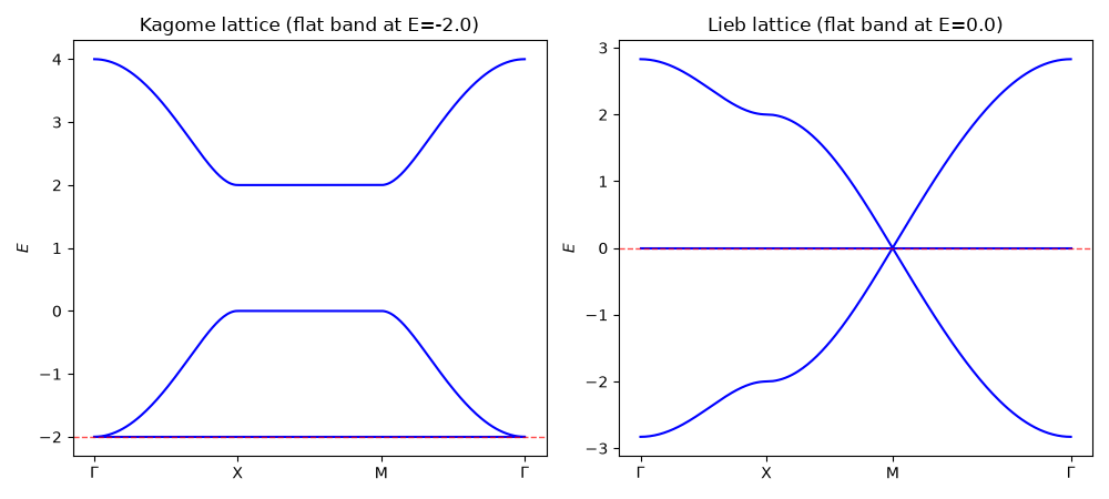
Kagome: flat band bandwidth = 3.55e-15 (should be ~0)
Lieb: flat band bandwidth = 0.00e+00 (should be ~0)