Landau Levels: Square Lattice vs. Graphene

A weak, uniform magnetic field (set_magnetic_field(), same Peierls substitution as the Aharonov-Bohm and Hofstadter-butterfly examples) quantizes a 2D band’s low-energy spectrum into discrete Landau levels. Two flakes, two very different ladders:

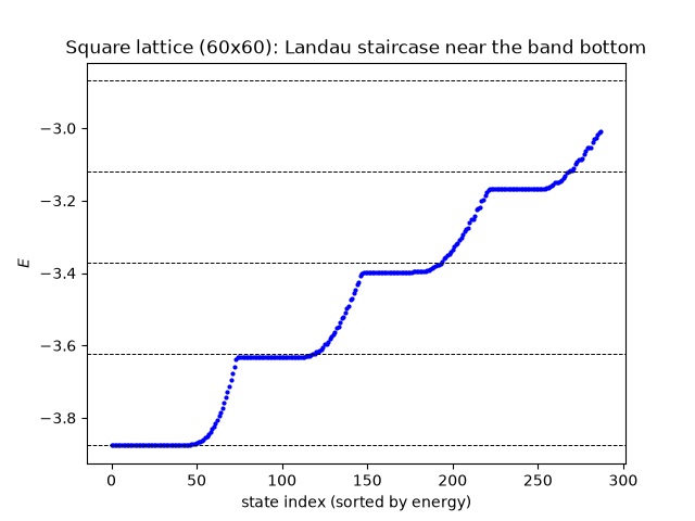
• A normal square lattice has a parabolic band bottom, so it reproduces the textbook non-relativistic Landau ladder, evenly spaced in energy,

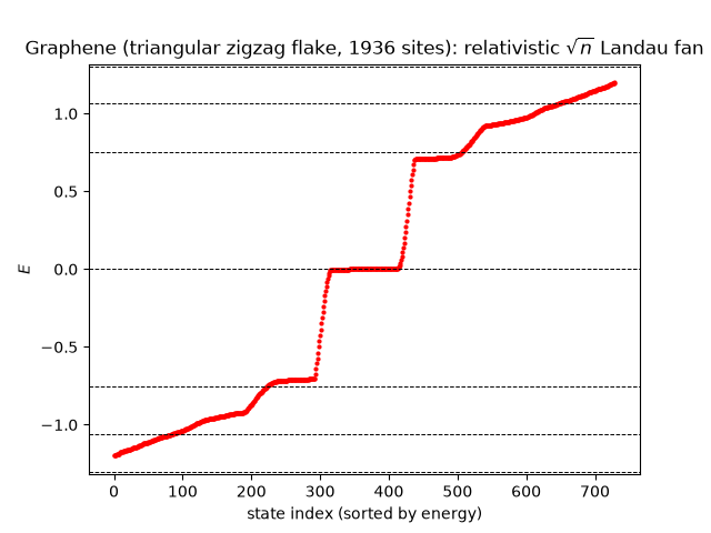
  \[E_n = E_0 + \hbar\omega_c\left(n+\tfrac12\right), \qquad n = 0,1,2,\dots\]

• Graphene’s linear (Dirac) dispersion instead gives the relativistic ladder, spaced by \(\sqrt{n}\) rather than \(n\), and pinned through an exact zero-energy level regardless of field strength – the signature that first confirmed graphene’s electrons behave as massless Dirac fermions (Novoselov et al., 2005; Zhang et al., 2005):

  \[E_n = \mathrm{sign}(n)\, v_F\sqrt{2\hbar e B|n|}, \qquad n = 0, \pm1, \pm2,\dots\]

import numpy as np
import matplotlib.pyplot as plt

from tbkit.lattice import Lattice
from tbkit.system import System
from tbkit.plot import Plot
from tbkit.graphene import GrapheneLattice


t = 1.
alpha = 0.02  # weak field: flux quanta per unit cell area

Square lattice: the non-relativistic Landau fan

Near the band bottom \(E\approx-4t+t(k_x^2+k_y^2)\), a square lattice looks exactly like a free particle of effective mass \(m^*=1/2t\), so weak-field Landau theory applies directly with \(\omega_c = 2t\cdot B = 4\pi t\alpha\) (\(\hbar=1\), \(\Phi_0=2\pi\), lattice constant 1).

# The two flakes the field is applied to, drawn small: a square lattice,
# whose parabolic band bottom gives the textbook ladder, and a graphene
# flake, whose Dirac cone gives the relativistic one. The flakes actually
# diagonalized below are much larger, so that the magnetic length fits
# comfortably inside them.
fig_lat, axes_lat = plt.subplots(1, 2, figsize=(9.5, 4.6))

lat_small = Lattice(unit_cell=[{'tag': 'a', 'r0': (0., 0.)}],
                              prim_vec=[(1., 0.), (0., 1.)])
lat_small.get_lattice(n1=10, n2=10)
sq_small = System(lat_small)
sq_small.set_hopping([{'n': 1, 't': t}])
Plot(sq_small).lattice(plt_hop=True, ms=8, ax=axes_lat[0])
axes_lat[0].set_title('square flake')

glat_small = GrapheneLattice()
glat_small.triangle_zigzag(n=8)
gsys_small = System(glat_small)
gsys_small.set_hopping([{'n': 1, 't': t}])
Plot(gsys_small).lattice(plt_hop=True, ms=8, ax=axes_lat[1])
axes_lat[1].set_title('graphene flake')

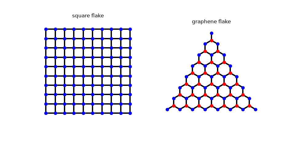
Text(0.5, 1.0, 'graphene flake')

The square lattice at full size:

N1, N2 = 60, 60
lat = Lattice(unit_cell=[{'tag': 'a', 'r0': (0., 0.)}], prim_vec=[(1., 0.), (0., 1.)])
lat.get_lattice(n1=N1, n2=N2)
sq = System(lat)
sq.set_hopping([{'n': 1, 't': t}])
sq.set_magnetic_field(alpha=alpha)
sq.get_ham()
sq.get_eig()
en_sq = np.sort(sq.en.real)

# The square lattice is bipartite, so its spectrum stays exactly
# symmetric under E -> -E even with the field on.
assert np.allclose(en_sq, -en_sq[::-1], atol=1e-8)
print('Square lattice: particle-hole symmetry E -> -E exact to machine precision.')

omega_c = 4 * np.pi * t * alpha
E0 = -4 * t
# A Landau level's degeneracy is exactly one state per flux quantum
# threading the flake.
degeneracy = round(alpha * N1 * N2)
lowest_level_mean = en_sq[:degeneracy].mean()
predicted_n0 = E0 + 0.5 * omega_c
print('Lowest Landau level (n=0): {} nearly-degenerate states, mean E={:.4f} '
           '(predicted {:.4f}).'.format(degeneracy, lowest_level_mean, predicted_n0))
assert abs(lowest_level_mean - predicted_n0) < 0.15 * omega_c

fig, ax = plt.subplots()
window = en_sq[en_sq < -3.]
ax.plot(window, 'o', ms=2, color='b')
for n in range(5):
    ax.axhline(E0 + omega_c * (n + 0.5), color='k', ls='--', lw=0.7)
ax.set_xlabel('state index (sorted by energy)')
ax.set_ylabel('$E$')
ax.set_title("Square lattice ({}x{}): Landau staircase near the band bottom".format(N1, N2))

Square lattice: particle-hole symmetry E -> -E exact to machine precision.
Lowest Landau level (n=0): 72 nearly-degenerate states, mean E=-3.8535 (predicted -3.8743).

Text(0.5, 1.0, 'Square lattice (60x60): Landau staircase near the band bottom')

Graphene: the relativistic Landau fan and the zero mode

A triangular zigzag flake keeps corner/edge-state weight well separated in energy from the bulk Landau ladder, which is what makes the plateaus below so clean. (The cluster right at E=0 is a mix of the field-induced n=0 Landau level and the flake’s own sublattice zero modes from Lieb’s theorem – see History, 1989.)

glat = GrapheneLattice()
glat.triangle_zigzag(n=44)
gsys = System(glat)
gsys.set_hopping([{'n': 1, 't': t}])
gsys.set_magnetic_field(alpha=alpha)
gsys.get_ham()
gsys.get_eig()
en_gr = np.sort(gsys.en.real)

assert np.allclose(en_gr, -en_gr[::-1], atol=1e-8)
print('\nGraphene flake: particle-hole symmetry E -> -E exact to machine precision.')

n_zero = np.sum(np.abs(en_gr) < 0.05)
print('n=0 manifold: {} states with |E|<0.05 (field-induced zero Landau level '
           '+ intrinsic sublattice zero modes).'.format(n_zero))
assert n_zero > 0

v_F = 1.5 * t  # Wallace's 1947 result, see :doc:`plot_graphene_bands`
B = 2 * np.pi * alpha
predicted_n1 = v_F * np.sqrt(2 * B)
plateau = en_gr[(en_gr > 0.6) & (en_gr < 0.9)]
print('n=1 Landau level: {} states, mean E={:.4f} (predicted {:.4f}).'
           .format(len(plateau), plateau.mean(), predicted_n1))
assert len(plateau) > 20
assert abs(plateau.mean() - predicted_n1) < 0.1 * predicted_n1

fig2, ax2 = plt.subplots()
window_gr = en_gr[np.abs(en_gr) < 1.2]
ax2.plot(window_gr, 'o', ms=2, color='r')
for n in range(-3, 4):
    predicted = np.sign(n) * v_F * np.sqrt(2 * B * abs(n)) if n else 0.
    ax2.axhline(predicted, color='k', ls='--', lw=0.7)
ax2.set_xlabel('state index (sorted by energy)')
ax2.set_ylabel('$E$')
ax2.set_title('Graphene (triangular zigzag flake, {} sites): '
                        r'relativistic $\sqrt{{n}}$ Landau fan'.format(glat.sites))

Graphene flake: particle-hole symmetry E -> -E exact to machine precision.
n=0 manifold: 106 states with |E|<0.05 (field-induced zero Landau level + intrinsic sublattice zero modes).
n=1 Landau level: 102 states, mean E=0.7452 (predicted 0.7520).

Text(0.5, 1.0, 'Graphene (triangular zigzag flake, 1936 sites): relativistic $\\sqrt{n}$ Landau fan')