Majorana Nanowires: Rashba, Zeeman and s-Wave Pairing

Kitaev’s chain needs spinless fermions with p-wave pairing, which no material offers. In 2010 R. Lutchyn, J. Sau and S. Das Sarma, and independently Y. Oreg, G. Refael and F. von Oppen, built one from ordinary parts: a semiconductor nanowire with strong Rashba spin-orbit coupling \(\alpha\), a Zeeman field \(V_Z\) perpendicular to the spin-orbit field, and s-wave pairing \(\Delta\) induced by a superconductor nearby,

\[H = \sum_j\Big[t\,c_j^\dagger c_{j+1} - i\alpha\,c_j^\dagger\sigma_y c_{j+1} + h.c.\Big] + \sum_j c_j^\dagger(V_Z\sigma_x - \mu)c_j + \Delta\sum_j\big(c_{j\uparrow}^\dagger c_{j\downarrow}^\dagger + h.c.\big)\, .\]

The field opens a gap between the two spin-orbit split bands; with the chemical potential in it, a single band is left at the Fermi level and the pairing it inherits is p-wave. The wire becomes topological when the gap at \(k = 0\) closes and reopens,

\[V_Z^2 > \Delta^2 + \mu_0^2\, ,\]

with \(\mu_0\) the chemical potential measured from the band bottom – and an open wire then binds a Majorana zero mode at each end. The zero-bias conductance peaks seen in such wires since 2012 (Mourik et al.) started the search for topological qubits.

The wire is an OrbitalSystem chain with set_rashba and set_zeeman, made superconducting by bdg_ham() with pairing_s_wave(); its periodic twin, a spinful KSpace through bdg_kspace(), gives Kitaev’s Majorana number.

import numpy as np
import matplotlib.pyplot as plt

import tbkit.lattices as lattices
from tbkit.bdg import bdg_ham, bdg_kspace, majorana_number, pairing_s_wave
from tbkit.kspace import KSpace, PAULI
from tbkit.orbital import OrbitalSystem
from tbkit.plot import Plot
from tbkit.system import System

t, alpha, delta = -1., 0.5, 0.3  # band bottom at mu = 2t = -2


def wire(n, vz, mu):
    '''BdG Hamiltonian of an open wire of n sites.'''
    lat = lattices.chain()
    lat.get_lattice(n)
    sys = OrbitalSystem(lat, spin=True)
    sys.set_hopping([{'n': 1, 't': t}])
    sys.set_rashba(alpha)  # -i alpha sigma_y on a bond along +x
    sys.set_zeeman((vz, 0., 0.))
    sys.get_ham()
    return bdg_ham(sys.ham, pairing_s_wave(n, delta), mu=mu).toarray()


def wire_bloch(vz, mu):
    '''The same wire, periodic: BdG Bloch Hamiltonian.'''
    ks = KSpace(lattices.chain(), spin=True)
    ks.set_hopping([{'i': 0, 'j': 0, 'R': (1,), 't': t * PAULI['0'] - 1j * alpha * PAULI['y']}])
    ks.set_onsite({'a': vz * PAULI['x']})
    return bdg_kspace(ks, [{'i': 0, 'j': 1, 'R': (0,), 'delta': delta}], mu=mu)

The lattice

The wire is a chain with one site per cell, each holding a spin-1/2 orbital. Each nearest-neighbour bond carries the hopping \(t\) and the Rashba spin-orbit coupling \(\alpha\); on each site act the Zeeman field \(V_z\) and the s-wave pairing \(\Delta\).

patch = lattices.chain()
patch.get_lattice(n1=10)
vis = System(patch)
vis.set_hopping([{'n': 1, 't': t}])
fig_lat = Plot(vis).lattice(plt_hop=True, ms=12, figsize=(7, 1.2))

The real-space and Bloch models agree

n = 60
for vz, mu in ((0.1, -2.), (0.6, -2.), (0.8, -1.5)):
    assert np.allclose(np.linalg.eigvalsh(wire(n, vz, mu)),
                              np.linalg.eigvalsh(wire_bloch(vz, mu).finite_ham(n)))

The phase diagram: the Majorana number against the gap closings

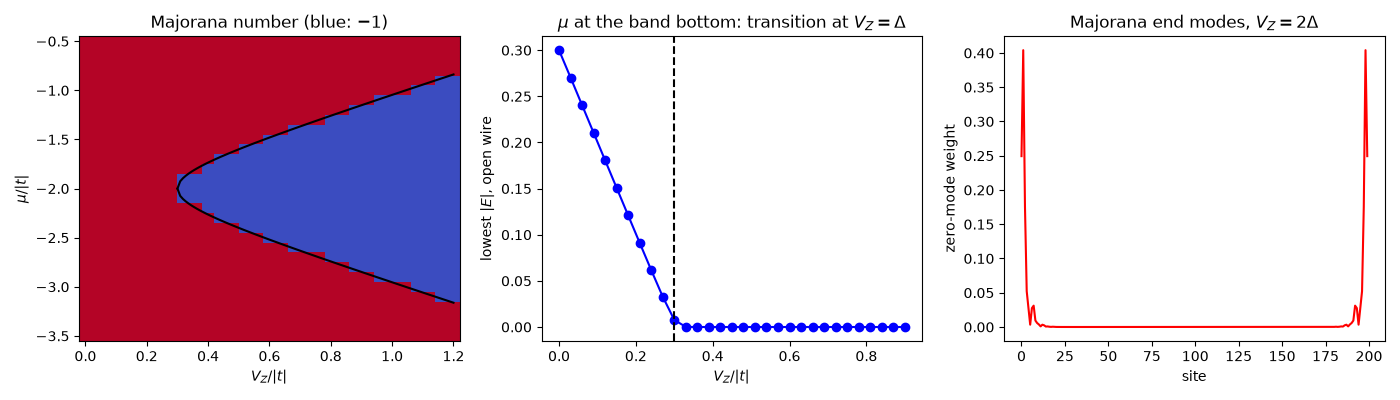
The gap can close only at k = 0 or \(\pi\) (where the Rashba term vanishes), when \(V_Z^2 = \Delta^2 + (\mu \mp 2t)^2\). The Majorana number is -1 between the two closings.

vzs = np.linspace(0., 1.2, 31)
mus = np.linspace(-3.5, -0.5, 31)
phase = np.full((len(mus), len(vzs)), np.nan)
for a, mu in enumerate(mus):
    for b, vz in enumerate(vzs):
        bottom = vz ** 2 - delta ** 2 - (mu - 2 * t) ** 2
        top = vz ** 2 - delta ** 2 - (mu + 2 * t) ** 2
        if min(abs(bottom), abs(top)) < 1e-6:
            continue  # gapless at a time-reversal-invariant momentum
        phase[a, b] = majorana_number(wire_bloch(vz, mu))
        assert phase[a, b] == (-1 if (bottom > 0) != (top > 0) else 1)
print('Majorana number = -1 exactly where V_Z^2 > Delta^2 + (mu - 2t)^2 (near the band bottom).')

Majorana number = -1 exactly where V_Z^2 > Delta^2 + (mu - 2t)^2 (near the band bottom).

Majorana zero modes at the ends of an open wire

At the band bottom (\(\mu = 2t\)) the criterion is \(V_Z > \Delta\). Below it the wire is gapped; above it two BdG states sit at zero energy, one at each end.

n, mu = 200, 2 * t
vz_scan = np.linspace(0., 0.9, 31)
lowest = np.array([np.sort(np.abs(np.linalg.eigvalsh(wire(n, vz, mu))))[0] for vz in vz_scan])
assert np.all(lowest[vz_scan < delta - 0.05] > 0.04)
assert np.all(lowest[vz_scan > delta + 0.15] < 1e-6)
en, vec = np.linalg.eigh(wire(n, 0.6, mu))
zero = np.argsort(np.abs(en))[:2]
assert np.max(np.abs(en[zero])) < 1e-10 and np.sort(np.abs(en))[2] > 0.2
# weight per site: particle and hole, both spins, both zero modes
weight = (np.abs(vec[:, zero]) ** 2).reshape(2, n, 2, 2).sum(axis=(0, 2, 3))
ends = (weight[:20].sum() + weight[-20:].sum()) / 2
print('V_Z = 0.6: two states at |E| < 1e-10; {:.1%} of their weight on the outer 20 sites.'.format(ends))
assert ends > 0.99

fig, axes = plt.subplots(1, 3, figsize=(14, 4))
axes[0].pcolormesh(vzs, mus, phase, cmap='coolwarm', shading='nearest')
fine = np.linspace(delta, 1.2, 100)
for sign in (1, -1):
    axes[0].plot(fine, 2 * t + sign * np.sqrt(fine ** 2 - delta ** 2), '-k')
axes[0].set_xlabel(r'$V_Z/|t|$')
axes[0].set_ylabel(r'$\mu/|t|$')
axes[0].set_title(r'Majorana number (blue: $-1$)')
axes[1].plot(vz_scan, lowest, 'o-b')
axes[1].axvline(delta, color='k', ls='--')
axes[1].set_xlabel(r'$V_Z/|t|$')
axes[1].set_ylabel(r'lowest $|E|$, open wire')
axes[1].set_title(r'$\mu$ at the band bottom: transition at $V_Z = \Delta$')
axes[2].plot(np.arange(n), weight, '-r')
axes[2].set_xlabel('site')
axes[2].set_ylabel('zero-mode weight')
axes[2].set_title(r'Majorana end modes, $V_Z = 2\Delta$')
fig.set_layout_engine('tight')

V_Z = 0.6: two states at |E| < 1e-10; 100.0% of their weight on the outer 20 sites.