The Photovoltaic Hall Effect in Graphene

Oka and Aoki (2009) asked what a DC field does to graphene that is illuminated by circularly polarized light, and found a Hall current with no magnetic field: the photovoltaic Hall effect. An electron near a Dirac point is driven around a circle in momentum space once per period, and the geometric (Aharonov-Anandan) phase it picks up acts as a Berry curvature of the Floquet states \(|u_\alpha(\mathbf{k})\rangle\). The Hall conductivity follows from the Floquet extension of the Kubo formula,

\[\sigma_{xy} = \frac{e^2}{h}\,\frac{1}{2\pi}\int d^2k\, \sum_\alpha f_\alpha(\mathbf{k})\,\Omega_\alpha(\mathbf{k})\, ,\]

with \(f_\alpha\) the occupations of the Floquet bands. Light gaps both Dirac points with a mass \(m\) (see the Floquet Chern insulator example), and the Berry curvature it creates has the same sign at \(K\) and \(K'\), so the two valleys add up instead of cancelling. That is the difference from a static staggered potential (Semenoff’s mass), which opens the same gap without any Hall response. With the lower Floquet band full, \(\sigma_{xy} = \pm e^2/h\); at a Fermi level \(E_F\) in the upper band, each valley is a massive Dirac cone and

\[|\sigma_{xy}| = \frac{e^2}{h}\,\frac{m}{|E_F|}\qquad (|E_F| > m)\, .\]

FloquetKSpace gives the Floquet bands, and berry_curvature() their curvature over the Brillouin zone.

import numpy as np
import matplotlib.pyplot as plt

import tbkit.lattices as lattices
from tbkit.bridges import finite_system
from tbkit.floquet import FloquetKSpace
from tbkit.kspace import KSpace, reciprocal_vectors
from tbkit.plot import Plot

graphene = KSpace(lattices.honeycomb())
graphene.set_hopping([{'i': 0, 'j': 1, 'R': R, 't': 1.} for R in [(0, 0), (-1, 0), (0, -1)]])
omega, a0 = 8., 0.8
driven = FloquetKSpace(graphene, lambda t: (a0 * np.cos(omega * t), a0 * np.sin(omega * t)),
                                2 * np.pi / omega, n_steps=20)
b1, b2 = (np.array(v) for v in reciprocal_vectors(graphene.lat.prim_vec))
K = (b1 - b2) / 3
mass = np.diff(np.linalg.eigvalsh(driven.get_ham(K)))[0] / 2
print('Light-induced mass at K: m = {:.4f}'.format(mass))

Light-induced mass at K: m = 0.1459

The lattice

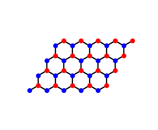
Graphene’s honeycomb lattice on a patch of \(5\times4\) cells (finite_system()): two sites per unit cell (sublattices ‘a’ and ‘b’, in two colours), each bonded to its three nearest neighbours on the other sublattice.

fig_lat = Plot(finite_system(graphene, (5, 4))).lattice(plt_hop=True, ms=12, figsize=(5.5, 4.5))

Berry curvature of the Floquet bands: both valleys alike

The plaquette fluxes of the lower band are split between the two valleys by their nearest Dirac point. A static staggered potential of the same mass gives the comparison. (The curvature is that of the periodic gauge, which can move some weight from one valley to the other but not change the total.)

nk = 90
curv = driven.berry_curvature(0, nk)
fracs = (np.indices((nk, nk)).reshape(2, -1).T + 0.5) / nk
centres = fracs @ np.array([b1, b2])
images = [i * b1 + j * b2 for i in (-1, 0, 1, 2) for j in (-1, 0, 1, 2)]


def distance(point):
    return np.min([np.linalg.norm(centres - point - g, axis=1) for g in images], axis=0)


near_k = distance(K) < distance(-K)


def valley_fluxes(c):
    c = c.ravel()
    return c[near_k].sum() / (2 * np.pi), c[~near_k].sum() / (2 * np.pi)


semenoff = KSpace(lattices.honeycomb())
semenoff.set_hopping([{'i': 0, 'j': 1, 'R': R, 't': 1.} for R in [(0, 0), (-1, 0), (0, -1)]])
semenoff.set_onsite({'a': mass, 'b': -mass})
light_k, light_kp = valley_fluxes(curv)
static_k, static_kp = valley_fluxes(semenoff.berry_curvature(0, nk))
print("Lower-band Berry flux / 2 pi at K and K': light {:+.3f}, {:+.3f}; staggered potential {:+.3f}, {:+.3f}"
          .format(light_k, light_kp, static_k, static_kp))
assert np.sign(light_k) == np.sign(light_kp) and min(abs(light_k), abs(light_kp)) > 0.4
assert np.isclose(abs(light_k + light_kp), 1., atol=1e-6)
assert np.sign(static_k) != np.sign(static_kp) and min(abs(static_k), abs(static_kp)) > 0.4
assert np.isclose(static_k + static_kp, 0., atol=1e-6)

Lower-band Berry flux / 2 pi at K and K': light -0.536, -0.464; staggered potential +0.442, -0.442

The Hall conductivity at any filling of the Floquet bands

The two curvatures of a two-band model add up to zero on every plaquette, so the upper band’s is minus the lower one’s.

en = driven.mesh_bands(nk).reshape(nk, nk, 2)


def hall(e_fermi):
    occupied = (en[..., 0] < e_fermi).astype(float) - (en[..., 1] < e_fermi)
    return np.sum(curv * occupied) / (2 * np.pi)


sigma_gap = hall(0.)
ratios = np.array([1.25, 1.5, 2.])
sigma_band = np.array([hall(r * mass) for r in ratios])
print('sigma_xy (e^2/h): {:+.4f} in the gap; |sigma| = {} at E_F / m = {}, m / E_F = {}'
          .format(sigma_gap, np.round(np.abs(sigma_band), 3), ratios, np.round(1 / ratios, 3)))
assert np.isclose(abs(sigma_gap), 1., atol=1e-6)
assert np.allclose(np.abs(sigma_band), 1 / ratios, rtol=0.05)
assert np.all(np.sign(sigma_band) == np.sign(sigma_gap))

fig, axes = plt.subplots(1, 2, figsize=(11, 4.4))
cart = (np.indices((nk, nk)).reshape(2, -1).T / nk) @ np.array([b1, b2])
lim = np.max(np.abs(curv))
sc = axes[0].scatter(cart[:, 0], cart[:, 1], c=curv.ravel(), s=4, cmap='RdBu_r', vmin=-lim, vmax=lim)
axes[0].set_aspect('equal')
axes[0].set_xlabel('$k_x$')
axes[0].set_ylabel('$k_y$')
axes[0].set_title('lower Floquet band: Berry flux per plaquette')
fig.colorbar(sc, ax=axes[0])
e_f = np.linspace(-4 * mass, 4 * mass, 161)
axes[1].plot(e_f / mass, [hall(e) for e in e_f], 'b', label='Floquet bands of graphene')
dirac = np.where(np.abs(e_f) > mass, np.sign(sigma_gap) * mass / np.maximum(np.abs(e_f), mass), np.nan)
axes[1].plot(e_f / mass, dirac, 'k--', lw=1,
                 label=r'massive Dirac cones, $m/|E_F|$')
axes[1].set_xlabel(r'$E_F / m$')
axes[1].set_ylabel(r'$\sigma_{xy}$ ($e^2/h$)')
axes[1].set_title('photovoltaic Hall conductivity')
axes[1].legend(fontsize=8)
fig.set_layout_engine('tight')

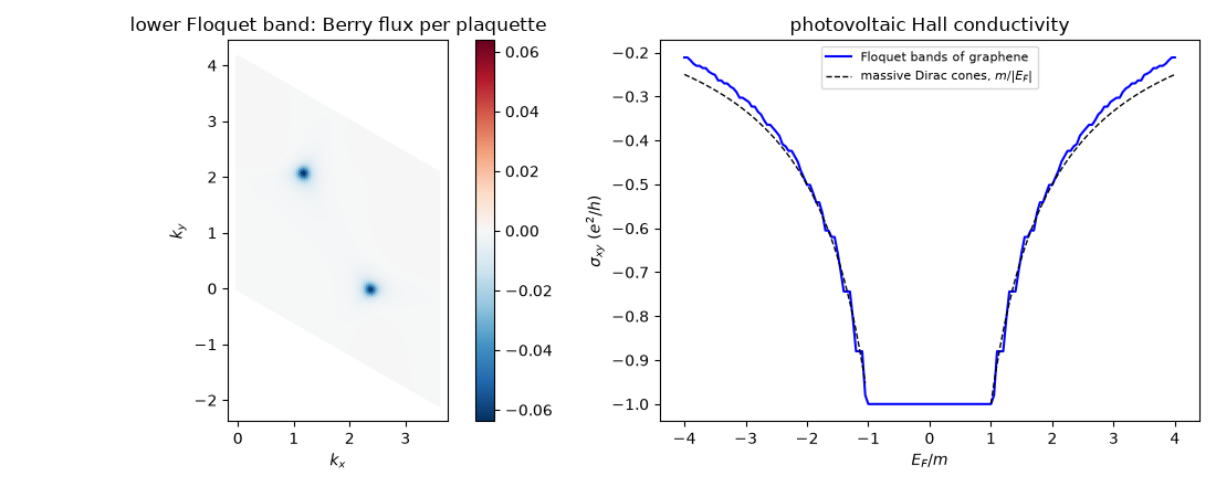
sigma_xy (e^2/h): -1.0000 in the gap; |sigma| = [0.807 0.656 0.501] at E_F / m = [1.25 1.5  2.  ], m / E_F = [0.8   0.667 0.5  ]