The BCS Gap Equation: Delta(T) and the Universal Ratio Delta(0)/T_c = 1.764

J. Bardeen, L. Cooper and J. R. Schrieffer (1957) explained superconductivity by the pairing of electrons with opposite momenta and spins into a condensate, whose gap \(\Delta\) solves the self-consistent gap equation

\[1 = \frac{V}{N}\sum_{\mathbf{k}}\frac{\tanh(E_{\mathbf{k}}/2T)}{2E_{\mathbf{k}}}\, , \qquad E_{\mathbf{k}} = \sqrt{\xi_{\mathbf{k}}^2 + \Delta^2}\, .\]

At weak coupling its solution is universal: \(\Delta(T)\) falls from \(\Delta(0)\) to zero at \(T_c\), as \(\sqrt{1 - T/T_c}\) near \(T_c\), with \(\Delta(0) = 1.764\,k_BT_c\) whatever the material.

In real space the same equation is the self-consistency of the Bogoliubov-de Gennes Hamiltonian, \(\Delta_i = V\langle c_{i\downarrow}c_{i\uparrow}\rangle\) on every site (tbkit.bdg.s_wave_gap()), which also handles inhomogeneous systems. Here: a clean \(12\times12\) square-lattice torus (\(t = 1\), \(\mu = -0.5\), \(V = 2.5\)), and a chain whose attraction stops halfway.

import numpy as np
import matplotlib.pyplot as plt
from scipy.optimize import brentq

import tbkit.lattices as lattices
from tbkit.bdg import s_wave_gap
from tbkit.bridges import finite_system
from tbkit.kspace import KSpace
from tbkit.plot import Plot

sq = KSpace(lattices.square())
sq.set_hopping([{'i': 0, 'j': 0, 'R': (1, 0), 't': -1.}, {'i': 0, 'j': 0, 'R': (0, 1), 't': -1.}])
L, mu, V = 12, -0.5, 2.5
h = sq.finite_ham(L, periodic=True).real
xi = sq.mesh_bands(L)[:, 0] - mu


def bcs(T):
    '''The k-space gap equation on the same 12 x 12 mesh.'''
    def eq(d):
        e = np.sqrt(xi**2 + d**2)
        return V / len(xi) * np.sum((np.tanh(e / (2 * T)) if T > 0 else 1.) / (2 * e)) - 1
    return brentq(eq, 1e-9, 5.) if eq(1e-9) > 0 else 0.

The lattice

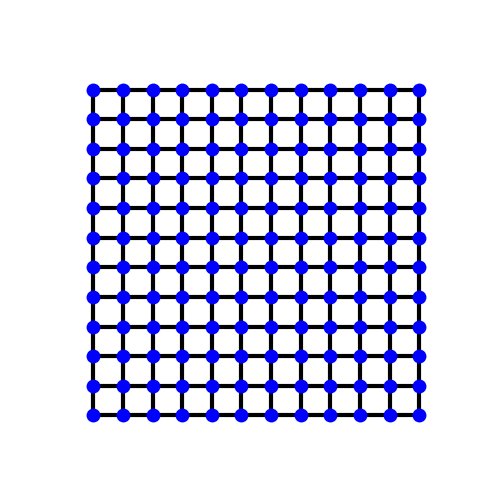
The square lattice, one site per cell with a nearest-neighbour hopping, as the \(12\times12\) torus solved below (finite_system(); the bonds that close the torus are not drawn). The attraction \(V\) acts on each site.

fig_lat = Plot(finite_system(sq, (L, L))).lattice(plt_hop=True, ms=10, figsize=(5, 5))

Delta(T) in real space

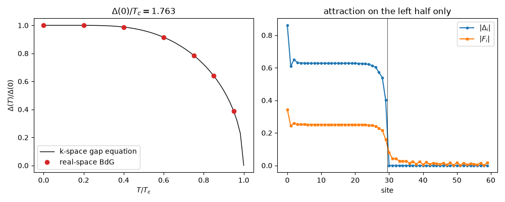
The real-space solution is uniform and equals the k-space one. T_c, from the linear vanishing of \(\Delta^2\), agrees with the linearized gap equation, and \(\Delta(0)/T_c = 1.764\) to 2%.

tc = brentq(lambda T: V / len(xi) * np.sum(np.tanh(xi / (2 * T)) / (2 * xi)) - 1, 1e-3, 3.)
d0 = s_wave_gap(h, V, mu).mean_gap
temps = np.array([0.2, 0.4, 0.6, 0.75, 0.85, 0.95]) * tc
gaps = []
for T in temps:
    res = s_wave_gap(h, V, mu, temperature=float(T), delta0=d0)
    assert np.allclose(np.abs(res.delta), res.mean_gap, atol=1e-7)
    assert abs(res.mean_gap - bcs(T)) < 1e-6
    gaps.append(res.mean_gap)
gaps = np.array(gaps)
tc_fit = temps[-2] - gaps[-2]**2 * (temps[-1] - temps[-2]) / (gaps[-1]**2 - gaps[-2]**2)
assert abs(tc_fit / tc - 1) < 0.01 and abs(d0 / tc_fit - 1.764) < 0.02 * 1.764
print('Delta(0) = {:.4f}, T_c = {:.4f} (linearized: {:.4f}), Delta(0)/T_c = {:.3f}'
      .format(d0, tc_fit, tc, d0 / tc_fit))

Delta(0) = 0.5438, T_c = 0.3085 (linearized: 0.3062), Delta(0)/T_c = 1.763

The proximity effect

A chain with the attraction on its left half only: the pair amplitude \(F_i = \langle c_{i\downarrow}c_{i\uparrow}\rangle\) leaks into the normal half, where \(\Delta_i = V_iF_i\) vanishes.

n = 60
chain = -(np.eye(n, k=1) + np.eye(n, k=-1))
v_i = np.where(np.arange(n) < n // 2, 2.5, 0.)
prox = s_wave_gap(chain, v_i, 0.3, mixing=0.7, delta0=np.full(n, 0.3 + 0j))
en, vec = prox.energies, prox.states
pos = en > 0
pair = np.einsum('in,in->i', vec[:n, pos], vec[n:, pos].conj())
assert np.allclose(prox.delta[n // 2:], 0.) and abs(pair[n // 2 + 2]) > 1e-3

fig, axes = plt.subplots(1, 2, figsize=(10, 4))
t_line = np.linspace(0., 1., 60) * tc
axes[0].plot(t_line / tc, [bcs(T) / d0 for T in t_line], 'k-', lw=1, label='k-space gap equation')
axes[0].plot(np.concatenate([[0.], temps]) / tc, np.concatenate([[d0], gaps]) / d0, 'o',
                  c='C3', label='real-space BdG')
axes[0].set_xlabel('$T/T_c$')
axes[0].set_ylabel(r'$\Delta(T)/\Delta(0)$')
axes[0].set_title(r'$\Delta(0)/T_c = {:.3f}$'.format(d0 / tc_fit))
axes[0].legend()
axes[1].plot(np.abs(prox.delta), 'o-', ms=3, label=r'$|\Delta_i|$')
axes[1].plot(np.abs(pair), 's-', ms=3, label=r'$|F_i|$')
axes[1].axvline(n // 2 - 0.5, c='k', lw=0.5)
axes[1].set_xlabel('site')
axes[1].set_title('attraction on the left half only')
axes[1].legend()
fig.tight_layout()