Wave Propagation: Interference on a Ring and a Trapped Domain-Wall State

Propagation evolves a state in time (Crank-Nicolson, \(\hbar = 1\)). Two classic effects of lattice waves:

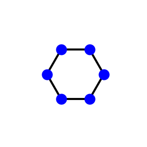
• Interference on a ring. On a hexagonal ring, a particle started on one site reaches the opposite site along two paths. Flip the sign of one hopping – a \(\pi\) flux through the ring – and the two paths cancel exactly: the opposite site is never reached (Aharonov-Bohm caging).

• A trapped state. A dimerized chain with a domain wall (the strong and weak bonds swap) binds a zero mode at the wall. A particle started there mostly stays: its long-time return probability is the sum \(\sum_n|\langle n|\psi_0\rangle|^4\) over the eigenstates, far larger than on a uniform chain, where it spreads away.

(This script replaces the pre-0.2 notebook examples_propagation.ipynb.)

import numpy as np
import matplotlib.pyplot as plt

from tbkit.lattice import Lattice
from tbkit.plot import Plot
from tbkit.propagation import Propagation
from tbkit.system import System

A hexagonal ring, with and without a pi flux

angles = np.arange(6) * np.pi / 3
ring_cell = [{'tag': 'a', 'r0': (float(np.cos(a)), float(np.sin(a)))} for a in angles]

# Six sites on a ring, each bond a hopping t = 1. A walker starting on the
# left-most site reaches the right-most one along two paths, one per arm.
ring = Lattice(unit_cell=ring_cell, prim_vec=[(10., 0.), (0., 10.)])
ring.get_lattice(n1=1, n2=1)
vis = System(ring)
vis.set_hopping([{'n': 1, 't': 1.}])
fig_ring = Plot(vis).lattice(plt_hop=True, ms=16, figsize=(3, 3))

The weight on the opposite site, without and with a \(\pi\) flux through the ring:

fig, axes = plt.subplots(1, 3, figsize=(13, 3.8))
far = {}
for flux in (False, True):
    lat = Lattice(unit_cell=ring_cell, prim_vec=[(10., 0.), (0., 10.)])
    lat.get_lattice(n1=1, n2=1)
    sys = System(lat)
    sys.set_hopping([{'n': 1, 't': 1.}])
    start = int(np.argmin(lat.coor['x']))
    opposite = int(np.argmax(lat.coor['x']))
    if flux:
        i, j = int(sys.hop['i'][0]), int(sys.hop['j'][0])
        sys.set_hopping_def({(i, j): -1.})
    sys.get_ham()
    prop = Propagation(lat)
    psi = np.zeros(lat.sites, 'c16')
    psi[start] = 1.
    prop.get_propagation(sys.ham, psi, steps=400, dz=0.05)
    weight = np.abs(prop.prop[opposite]) ** 2
    far[flux] = weight
    t = np.arange(prop.steps) * prop.dz
    axes[0].plot(t, weight, label=r'$\pi$ flux' if flux else 'no flux')
assert far[False].max() > 0.3 and far[True].max() < 1e-12
print('largest weight on the opposite site: {:.3f} (no flux), {:.1e} (pi flux)'.format(
    far[False].max(), far[True].max()))
axes[0].set_xlabel('time')
axes[0].set_ylabel('weight on the opposite site')
axes[0].set_title('hexagonal ring')
axes[0].legend()

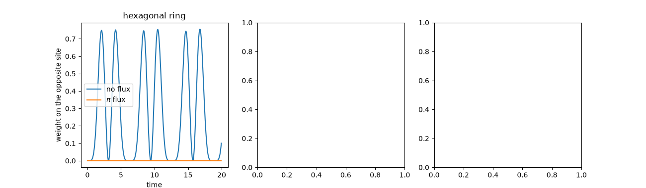
largest weight on the opposite site: 0.756 (no flux), 7.4e-32 (pi flux)

<matplotlib.legend.Legend object at 0x10f4dd7f0>

A domain wall in a dimerized chain

def dimer_chain(wall):
    lat = Lattice(unit_cell=[{'tag': 'a', 'r0': (0., 0.)}, {'tag': 'b', 'r0': (1., 0.)}],
                       prim_vec=[(2., 0.)])
    lat.get_lattice(n1=20)
    lat.remove_sites([39])
    sys = System(lat)
    sys.set_hopping([{'n': 1, 'tag': 'ab', 't': 2.}, {'n': 1, 'tag': 'ba', 't': 1.}])
    if wall:
        # swap the strong and weak bonds right of x = 20: a wall at site 20
        sys.change_hopping_square([{'n': 1, 'tag': 'ab', 't': 1.}, {'n': 1, 'tag': 'ba', 't': 2.}],
                                  xlims=[20., 40.])
    else:
        sys.set_hopping([{'n': 1, 'tag': 'ab', 't': 1.5}, {'n': 1, 'tag': 'ba', 't': 1.5}])
    sys.get_ham()
    return lat, sys

The chain with its domain wall, bond widths proportional to the hopping: strong bonds start each dimer left of site 20 (‘a’ to ‘b’) and right of it (‘b’ to ‘a’), so site 20 sits between two weak bonds.

fig_wall = Plot(dimer_chain(True)[1]).lattice(plt_hop=True, ms=6, c=2.5, figsize=(12, 1.2))

The return probability of a walker started on site 20:

for ax, wall in zip(axes[1:], (True, False)):
    lat, sys = dimer_chain(wall)
    site = 20
    prop = Propagation(lat)
    psi = np.zeros(lat.sites, 'c16')
    psi[site] = 1.
    prop.get_propagation(sys.ham, psi, steps=3000, dz=0.05)
    ret = np.abs(prop.prop[site]) ** 2
    en, vec = np.linalg.eigh(sys.ham.toarray())
    expected = np.sum(np.abs(vec[site]) ** 4)
    late = ret[1000:].mean()
    assert abs(late - expected) < 0.05
    if wall:
        assert np.min(np.abs(en)) < 1e-6 and late > 0.3
    else:
        assert late < 0.1
    print('{}: long-time return probability {:.3f} (eigenstate sum {:.3f})'.format(
        'domain wall' if wall else 'uniform chain', late, expected))
    ax.imshow(np.abs(prop.prop[:, ::10]) ** 2, aspect='auto', origin='lower', cmap='magma',
                  extent=[0, prop.steps * prop.dz, 0, lat.sites], vmax=0.3)
    ax.set_xlabel('time')
    ax.set_ylabel('site')
    ax.set_title('domain wall' if wall else 'uniform chain')
fig.tight_layout()

domain wall: long-time return probability 0.367 (eigenstate sum 0.366)
uniform chain: long-time return probability 0.038 (eigenstate sum 0.038)