The Intrinsic Spin Hall Effect: Kane-Mele Plateau and Rashba Coupling

An electric field along \(y\) can drive a spin current along \(x\) with no charge current at all: up and down spins are deflected to opposite sides. Murakami, Nagaosa and Zhang (2003) and Sinova et al. (2004) showed that spin-orbit coupling alone produces it, as a property of the band structure – the spin analogue of the intrinsic anomalous Hall effect. With the spin current \(j^s_x = \{s_z, v_x\}/2\), the Kubo formula gives the spin Hall conductivity (spin_hall_conductivity()), in units of \(e/2\pi\).

In the Kane-Mele model of graphene, intrinsic spin-orbit coupling \(\lambda_{SO}\) makes each spin a Haldane model, with opposite Chern numbers \(C_\uparrow = -C_\downarrow\). The charge Hall conductivity vanishes (time reversal), but, as long as \(s_z\) is conserved, the spin Hall conductivity in the gap is quantized: \(\sigma^s_{xy} = \frac{e}{2\pi}\,\frac{C_\uparrow - C_\downarrow}{2}\). Rashba coupling \(\lambda_R\) mixes the spins: the plateau is no longer quantized, although the gap – and the \(\mathbb{Z}_2\) topological phase – survive.

import numpy as np
import matplotlib.pyplot as plt

import tbkit.lattices as lattices
from tbkit.bridges import finite_system
from tbkit.kspace import KSpace, PAULI
from tbkit.plot import Plot

NN = [(0, 0), (-1, 0), (0, -1)]
NNN = [(0, 1), (-1, 0), (1, -1)]  # a2, -a1, a1 - a2: 120 degrees apart


def kane_mele(lam_so, lam_r=0.):
    '''Kane-Mele model: t = 1, intrinsic spin-orbit lam_so, Rashba lam_r.'''
    lat = lattices.honeycomb()
    km = KSpace(lat, spin=True)
    km.set_hopping([{'i': 0, 'j': 1, 'R': R, 't': 1.} for R in NN])
    for R in NNN:
        km.set_hopping([{'i': 0, 'j': 0, 'R': R, 't': 1j*lam_so*PAULI['z']},
                                {'i': 1, 'j': 1, 'R': R, 't': -1j*lam_so*PAULI['z']}])
    tau = np.array([d['r0'] for d in lat.unit_cell])
    a = np.array(lat.prim_vec)
    for R in NN:
        d = tau[1] + R[0]*a[0] + R[1]*a[1] - tau[0]
        d = d / np.linalg.norm(d)
        # i lam_r (sigma x d)_z on the nearest-neighbour bonds
        km.set_hopping([{'i': 0, 'j': 1, 'R': R, 't': 1j*lam_r*(PAULI['x']*d[1] - PAULI['y']*d[0])}])
    return km


def haldane_sector(lam_so, spin):
    '''One spin sector of Kane-Mele without Rashba: a Haldane model, t2 = +-i lam_so.'''
    ks = KSpace(lattices.honeycomb())
    ks.set_hopping([{'i': 0, 'j': 1, 'R': R, 't': 1.} for R in NN])
    for R in NNN:
        ks.set_hopping([{'i': 0, 'j': 0, 'R': R, 't': 1j*spin*lam_so},
                                {'i': 1, 'j': 1, 'R': R, 't': -1j*spin*lam_so}])
    return ks


lam_so = 0.06

The lattice

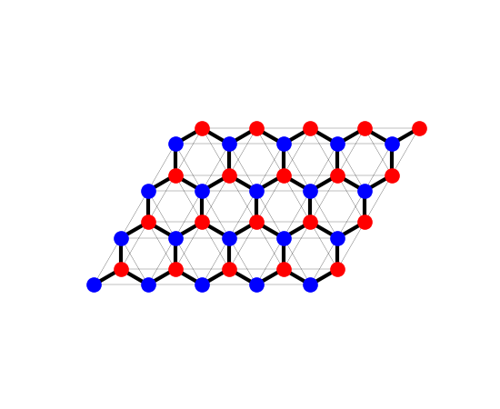
The Kane-Mele model without Rashba coupling is two copies of the Haldane model, one per spin. The spin-up copy on a patch of \(5\times4\) cells (finite_system()), bond widths proportional to the amplitudes: the honeycomb lattice’s two sublattices (‘a’ and ‘b’, in two colours), the nearest-neighbour hopping \(t\) (thick) and the spin-orbit hoppings \(\pm i\lambda_{SO}\) between second neighbours (thin). Spin down has the opposite signs.

fig_lat = Plot(finite_system(haldane_sector(lam_so, +1), (5, 4))).lattice(plt_hop=True, ms=12, figsize=(5.5, 4.5))

The quantized plateau, and the decoupled spin sectors

Without Rashba coupling, the two spins are two Haldane models. Their Chern numbers, from chern_number(), fix the plateau; in the bands, the spin Hall conductivity is half the difference of the two sectors’ Hall conductivities (each spin carries \(\pm\hbar/2\)).

km = kane_mele(lam_so)
up, down = haldane_sector(lam_so, +1), haldane_sector(lam_so, -1)
c_up, c_dn = up.chern_number([0], 40), down.chern_number([0], 40)
gap = 3 * np.sqrt(3) * lam_so  # half-gap at K and K'
e_f = np.linspace(-0.99, 0.99, 199)  # off the van Hove level |E| = 1, met exactly on the mesh
sigma_s = km.spin_hall_conductivity(e_f, nk=150)
sectors = (up.hall_conductivity(e_f, nk=150) - down.hall_conductivity(e_f, nk=150)) / 2
in_gap = np.abs(e_f) < gap - 0.02

print('C_up = {:.4f}, C_dn = {:.4f}; (C_up - C_dn)/2 = {:.4f}'.format(c_up, c_dn, (c_up - c_dn) / 2))
print('spin Hall plateau: {:.6f} to {:.6f} e/2pi'.format(sigma_s[in_gap].min(), sigma_s[in_gap].max()))
assert np.isclose(c_up, -c_dn, atol=1e-6) and np.isclose(abs(c_up), 1., atol=1e-6)
assert np.allclose(sigma_s[in_gap], (c_up - c_dn) / 2, atol=1e-6)
assert np.allclose(sigma_s, sectors, atol=1e-10)
# time reversal: no charge Hall current at any filling
assert np.max(np.abs(km.hall_conductivity(e_f, nk=60))) < 1e-12

C_up = 1.0000, C_dn = -1.0000; (C_up - C_dn)/2 = 1.0000
spin Hall plateau: 1.000000 to 1.000000 e/2pi

Rashba coupling breaks the quantization

With \(\lambda_R \neq 0\) the spin current is no longer conserved, and the value in the gap drifts away from \(e/2\pi\) – while the \(\mathbb{Z}_2\) invariant (z2_invariant()) stays 1: the gap stays open (it closes at \(\lambda_R = 2\sqrt3\,\lambda_{SO}\)). The values are converged in the mesh (150 x 150 against 300 x 300) to \(10^{-5}\).

rashba = [0., 0.05, 0.1]
curves, plateau = {}, []
for lam_r in rashba:
    model = kane_mele(lam_so, lam_r)
    curves[lam_r] = model.spin_hall_conductivity(e_f, nk=150)
    plateau.append(model.spin_hall_conductivity(0., nk=150))
    nu = model.z2_invariant([0, 1], nk=40, nk_perp=21)
    en = model.mesh_bands(150)
    print('lambda_R = {:.2f}: gap {:.3f}, sigma_s(E_F = 0) = {:.4f} e/2pi, Z2 = {}'.format(
        lam_r, en[:, 2].min() - en[:, 1].max(), plateau[-1], nu))
    assert nu == 1 and en[:, 2].min() - en[:, 1].max() > 0.3
    assert abs(plateau[-1] - model.spin_hall_conductivity(0., nk=300)) < 1e-5

deviation = np.abs(np.array(plateau) - plateau[0])
assert deviation[0] == 0. and np.all(np.diff(deviation) > 0) and deviation[-1] > 0.05

fig, ax = plt.subplots(figsize=(7, 4.5))
for lam_r, s in curves.items():
    ax.plot(e_f, s, label=r'$\lambda_R = {:.2f}$'.format(lam_r))
ax.plot(e_f, sectors, 'k:', lw=1, label=r'$(\sigma_\uparrow - \sigma_\downarrow)/2$, $\lambda_R = 0$')
ax.set_xlabel('$E_F$')
ax.set_ylabel(r'$\sigma^s_{xy}$ ($e/2\pi$)')
ax.set_title(r'Kane-Mele model, $\lambda_{SO} = 0.06$: spin Hall conductivity')
ax.legend()

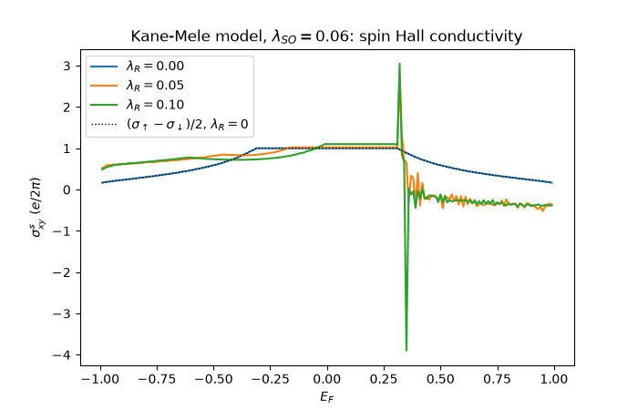
lambda_R = 0.00: gap 0.624, sigma_s(E_F = 0) = 1.0000 e/2pi, Z2 = 1
lambda_R = 0.05: gap 0.474, sigma_s(E_F = 0) = 1.0220 e/2pi, Z2 = 1
lambda_R = 0.10: gap 0.322, sigma_s(E_F = 0) = 1.0994 e/2pi, Z2 = 1

<matplotlib.legend.Legend object at 0x10f07d2b0>