The Tetrahedron Method for the Density of States

The density of states \(\rho(E) = \sum_n\int\frac{d\mathbf{k}}{V_{BZ}}\, \delta(E - E_n(\mathbf{k}))\) needs an integral over the Brillouin zone, but a calculation only knows the bands on a finite mesh. Broadening each eigenvalue into a Gaussian of width \(\sigma\) turns the sum into a smooth curve, at the price of smearing exactly the features that matter: band edges, and the van Hove singularities where \(\nabla_k E = 0\).

Jepsen and Andersen (1971) and Lehmann and Taut (1972) found the way out: split the zone into tetrahedra with mesh points at their corners, interpolate each band linearly inside every tetrahedron, and integrate the density of states of that interpolation exactly – it is a piecewise polynomial in \(E\), known in closed form. Blochl, Jepsen and Andersen (1994) gave the standard formulas. There is no \(\sigma\) to choose, and the error falls with the mesh instead of with a width.

tbkit.dos.tetrahedron_dos() implements the linear method in 1, 2 and 3 dimensions (segments, triangles, tetrahedra), and plot_dos() uses it with kernel='tetrahedron'.

import numpy as np
import matplotlib.pyplot as plt
from scipy.special import ellipk
from mpl_toolkits.mplot3d.art3d import Line3DCollection

import tbkit.dos as dos
import tbkit.lattices as lattices
from tbkit.lattice import Lattice
from tbkit.bridges import finite_system
from tbkit.kspace import KSpace
from tbkit.plot import Plot
from tbkit.system import System

The square lattice: a logarithmic van Hove singularity

\(E = -2(\cos k_x + \cos k_y)\) has saddle points at X, where the density of states diverges logarithmically. The exact result is \(\rho(E) = K(1 - E^2/16)/2\pi^2\) per site, with \(K\) the complete elliptic integral. On the same 80 x 80 mesh, the tetrahedron method is within 0.3% of it (away from the divergence itself), the Gaussian of width one mesh spacing in energy off by 6%.

sq = KSpace(lattices.square())
sq.set_hopping([{'i': 0, 'j': 0, 'R': (1, 0), 't': -1.}, {'i': 0, 'j': 0, 'R': (0, 1), 't': -1.}])

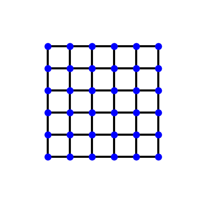
The square lattice, one site per cell with nearest-neighbour hopping, on \(6\times6\) cells (finite_system()):

fig_lat = Plot(finite_system(sq, (6, 6))).lattice(plt_hop=True, ms=10, figsize=(4, 4))

Its density of states, exact and on a mesh:

e_grid = np.linspace(-3.9, 3.9, 157)
exact = ellipk(1 - e_grid ** 2 / 16) / (2 * np.pi ** 2)
away = np.abs(e_grid) > 0.3

nk = 80
en = sq.mesh_bands(nk)
_, rho_tet = dos.tetrahedron_dos(en.reshape(nk, nk, 1), e_grid)
_, rho_gauss = dos.density_of_states(en, e_grid, broadening=8. / nk)
rho_tet, rho_gauss = rho_tet / nk ** 2, rho_gauss / nk ** 2  # per site
err_tet = np.abs(rho_tet - exact)[away].max() / exact[away].max()
err_gauss = np.abs(rho_gauss - exact)[away].max() / exact[away].max()
print('Square lattice, {0} x {0} mesh: tetrahedron error {1:.2%}, Gaussian error {2:.2%}'.format(
    nk, err_tet, err_gauss))
assert err_tet < 5e-3 and err_gauss > 5e-2

# the peak keeps growing with the mesh, like the logarithm it is
peaks = []
for n in (20, 40, 80):
    en_n = sq.mesh_bands(n).reshape(n, n, 1)
    peaks.append(dos.tetrahedron_dos(en_n, np.array([-0.01, 0., 0.01]))[1][1] / n ** 2)
print('rho(0) on 20, 40, 80 meshes:', np.round(peaks, 3))
assert peaks[0] < peaks[1] < peaks[2]

fig, ax = plt.subplots(figsize=(7, 4.5))
ax.plot(e_grid, exact, 'k', lw=3, label='exact')
ax.plot(e_grid, rho_gauss, 'r--', label=r'Gaussian, $\sigma = 0.1$')
ax.plot(e_grid, rho_tet, 'b', label='tetrahedron')
ax.set_ylim(0, 0.5)
ax.set_xlabel('$E/t$')
ax.set_ylabel(r'$\rho(E)$ per site')
ax.set_title('Square lattice, {0} x {0} k-points'.format(nk))
ax.legend()
fig.set_layout_engine('tight')

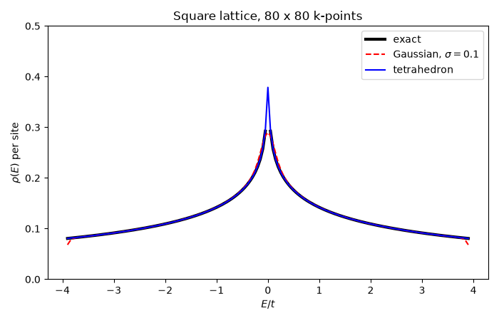
Square lattice, 80 x 80 mesh: tetrahedron error 0.26%, Gaussian error 6.21%
rho(0) on 20, 40, 80 meshes: [0.384 0.442 0.467]

The simple cubic lattice: band edges

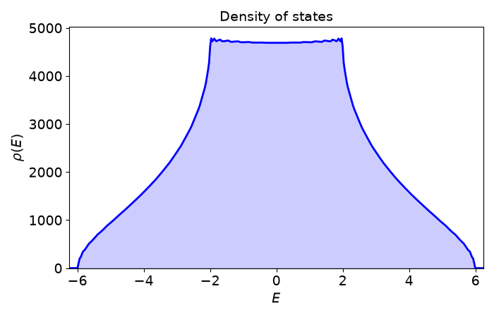
In 3D the density of states starts as \(\sqrt{E - E_0}\) at a band edge and has kinks (van Hove points) inside the band. The Gaussian leaks states below the band bottom \(E_0 = -6t\); the tetrahedron method puts none there, and converges to a 64 x 64 x 64 reference about ten times faster.

cubic = KSpace(Lattice(unit_cell=[{'tag': 'a', 'r0': (0., 0., 0.)}],
                              prim_vec=[(1., 0., 0.), (0., 1., 0.), (0., 0., 1.)]))
cubic.set_hopping([{'i': 0, 'j': 0, 'R': R, 't': -1.} for R in [(1, 0, 0), (0, 1, 0), (0, 0, 1)]])

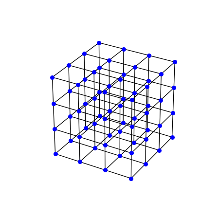
The simple cubic lattice, one site per cell and six nearest neighbours, here \(4\times4\times4\) sites of it:

lat_vis = Lattice(unit_cell=cubic.lat.unit_cell, prim_vec=cubic.lat.prim_vec)
lat_vis.get_lattice(4, 4, 4)
vis = System(lat_vis)
vis.set_hopping([{'n': 1, 't': 1.}])
pos = np.column_stack([lat_vis.coor[f] for f in 'xyz'])
bonds = np.stack([pos[vis.hop['i'].astype(int)], pos[vis.hop['j'].astype(int)]], axis=1)
fig_lat = plt.figure(figsize=(4.5, 4.5))
ax_lat = fig_lat.add_subplot(projection='3d')
ax_lat.add_collection3d(Line3DCollection(bonds, colors='k', linewidths=1))
ax_lat.scatter(*pos.T, s=30, c='b', depthshade=False)
ax_lat.set_aspect('equal')
ax_lat.set_axis_off()

Its density of states near the band bottom:

e_grid = np.linspace(-6.5, 6.5, 131)
ref = dos.tetrahedron_dos(cubic.mesh_bands(64).reshape(64, 64, 64, 1), e_grid)[1] / 64 ** 3

nk = 32
en = cubic.mesh_bands(nk)
rho_tet = dos.tetrahedron_dos(en.reshape(nk, nk, nk, 1), e_grid)[1] / nk ** 3
rho_gauss = dos.density_of_states(en, e_grid, broadening=12. / nk)[1] / nk ** 3
below = e_grid < -6.05
err_tet = np.abs(rho_tet - ref).max() / ref.max()
err_gauss = np.abs(rho_gauss - ref).max() / ref.max()
print('Simple cubic, 32^3 mesh: error {:.2%} (tetrahedron), {:.2%} (Gaussian)'.format(err_tet, err_gauss))
print('States below the band bottom: {:.1e} (tetrahedron), {:.1e} (Gaussian)'.format(
    rho_tet[below].max(), rho_gauss[below].max()))
assert err_tet < 1e-2 and err_gauss > 5e-2
assert rho_tet[below].max() == 0. and rho_gauss[below].max() > 1e-3
# one state per site in all
assert np.isclose(np.sum(rho_tet) * (e_grid[1] - e_grid[0]), 1.)

Simple cubic, 32^3 mesh: error 0.53% (tetrahedron), 9.71% (Gaussian)
States below the band bottom: 0.0e+00 (tetrahedron), 4.9e-03 (Gaussian)

The same in one call: plot_dos() with kernel='tetrahedron' (no broadening to choose).

fig2 = cubic.plot_dos(nk=32, kernel='tetrahedron', fs=14, figsize=(7, 4.5))