Completing Lead Interfaces: a Graphene Disc between Zigzag Leads

attach_lead() couples a lead to the outermost of its cells that the device reaches, and that cell must hold every lead orbital with a hopping into the lead. A device whose edge is ragged relative to the lead, such as a disc under a strip, does not end with such a cell.

attach_lead(..., extend=True) completes it, as Kwant’s attach_lead does. Starting from the lead’s first cell, it follows the lead’s hoppings towards the device and adds every lead site it reaches that the device lacks, until all the sites it reaches are present. The added sites carry the lead’s onsite energies and hoppings. They come after the device’s sites, and the method returns the enlarged Hamiltonian and the positions of all the sites.

import numpy as np
import matplotlib.pyplot as plt

import tbkit.lattices as lattices
from tbkit.kspace import ribbon
from tbkit.lattice import Lattice
from tbkit.system import System
from tbkit.transport import Transport, lead_from_kspace, lead_modes


def device(lat, keep, t):
    '''A System of the sites of *lat* selected by keep(x, y), nearest-neighbour hopping t.'''
    lat.coor = lat.coor[keep(lat.coor['x'], lat.coor['y'])]
    lat.sites = len(lat.coor)
    sys = System(lat)
    sys.set_hopping([{'n': 1, 't': t}])
    sys.get_ham()
    return sys


def positions(sys):
    return np.stack([sys.lat.coor['x'], sys.lat.coor['y']], axis=1)

A ragged rectangle gives back the full one

Remove a few sites from the ends of a square-lattice strip, then attach strip leads with extend=True. The sites put back are the missing ones, with the same hoppings: the enlarged Hamiltonian is the full strip’s (up to the order of the sites), and so is the transmission.

t, width, length = -1., 5, 8
square = [{'i': 0, 'j': 0, 'R': (1, 0), 't': t}, {'i': 0, 'j': 0, 'R': (0, 1), 't': t}]
strip = ribbon(lattices.square(), square, width=width, direction=1)


def rectangle(missing=()):
    lat = lattices.square()
    lat.get_lattice(length, width)
    return device(lat, lambda x, y: np.array([(a, b) not in missing for a, b in zip(x, y)]), t)


full = rectangle()
reference = Transport(full.ham)
reference.attach_lead(full, strip, -1)
reference.attach_lead(full, strip, 1)

missing = {(0., 3.), (0., 4.), (7., 0.), (7., 1.), (6., 0.)}
ragged = rectangle(missing)
tr = Transport(ragged.ham)
tr.attach_lead(ragged, strip, -1, extend=True)
ham, pos = tr.attach_lead(ragged, strip, 1, extend=True)

added = pos[ragged.lat.sites:]
assert {tuple(p) for p in added} == missing
order = [int(np.flatnonzero(np.all(np.isclose(positions(full), p), axis=1))[0]) for p in pos]
assert np.allclose(ham.toarray(), full.ham.toarray()[np.ix_(order, order)])
energies = np.linspace(-3.9, 3.9, 25)
assert np.allclose(tr.transmission(energies), reference.transmission(energies), atol=1e-8)
print('Ragged strip: the 5 missing sites are put back; H and T(E) are the full strip\'s.')

Ragged strip: the 5 missing sites are put back; H and T(E) are the full strip's.

A graphene disc between zigzag leads

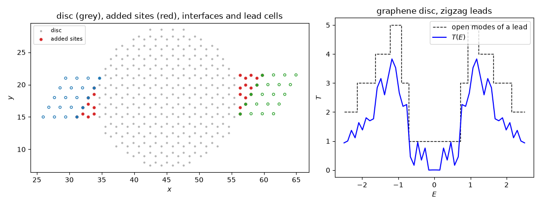
A disc of graphene and two zigzag ribbons along x, narrower than the disc, placed on its lattice. Without extend, attach_lead refuses the round edge. With it, the lead’s rows are filled in up to the disc on each side.

t = -1.
honeycomb = lattices.honeycomb()
lat = lattices.honeycomb()
lat.get_lattice(40, 24)
center = 20 * np.array(honeycomb.prim_vec[0]) + 12 * np.array(honeycomb.prim_vec[1])
radius = 11.
disc = device(lat, lambda x, y: np.hypot(x - center[0], y - center[1]) < radius, t)

# the zigzag ribbon, its rows moved onto rows of the disc's lattice
w_lead = 5
graphene = [{'i': 0, 'j': 1, 'R': (0, 0), 't': t}, {'i': 1, 'j': 0, 'R': (1, 0), 't': t},
            {'i': 1, 'j': 0, 'R': (0, 1), 't': t}]
a1, a2 = np.array(honeycomb.prim_vec)
row0 = int(np.rint((center[1] - 3.5) / a2[1])) * a2  # a lattice vector: rows stay on the lattice
zigzag = ribbon(Lattice(unit_cell=[{'tag': c['tag'], 'r0': tuple(np.array(c['r0']) + row0)}
                                   for c in honeycomb.unit_cell], prim_vec=honeycomb.prim_vec),
                graphene, width=w_lead, direction=1)

tr = Transport(disc.ham)
try:
    tr.attach_lead(disc, zigzag, -1)
except ValueError:
    print('Without extend, attach_lead refuses the round edge of the disc.')
else:
    raise AssertionError('the disc edge should be incomplete for the zigzag lead')
tr.attach_lead(disc, zigzag, -1, extend=True)
ham, pos = tr.attach_lead(disc, zigzag, 1, extend=True)
n_added = len(pos) - disc.lat.sites
assert n_added > 0 and ham.shape == (len(pos), len(pos))

# every added site sits on the honeycomb lattice, outside the disc, and
# has the bonds of graphene: one added or disc site at each neighbour
# position that is occupied
added = pos[disc.lat.sites:]
assert np.all(np.hypot(*(added - center).T) >= radius)
dist = np.linalg.norm(pos[:, None] - pos[None], axis=2)
bonds = np.abs(ham.toarray()) > 1e-12
assert np.array_equal(bonds, np.isclose(dist, 1.))
assert np.allclose(ham.toarray()[bonds], t)
print('Disc: {} sites added at the two contacts, all bonds those of graphene.'.format(n_added))

Without extend, attach_lead refuses the round edge of the disc.
Disc: 25 sites added at the two contacts, all bonds those of graphene.

Through the completed interfaces, the scattering matrix is unitary and the transmission is bounded by the open modes of the zigzag leads (the number of crossings of each energy with the ribbon’s bands).

energies = np.linspace(-2.5, 2.5, 50)  # avoids E = 0, the flat edge band
T = tr.transmission(energies)
h0, v = lead_from_kspace(zigzag)
modes = np.array([len(lead_modes(h0, v, e).momenta) // 2 for e in energies])
assert np.all(T <= modes + 1e-6) and np.all(T >= -1e-10)
for e in (-1.3, 0.4, 1.7):
    s = tr.smatrix(e)
    assert np.allclose(s.data.conj().T @ s.data, np.eye(s.data.shape[1]), atol=1e-8)
print('T(E) <= open modes of the zigzag leads; S is unitary.')

fig, (ax0, ax1) = plt.subplots(1, 2, figsize=(11, 4.2), width_ratios=(1.4, 1))
ax0.scatter(*positions(disc).T, s=4, c='0.7', label='disc')
ax0.scatter(*added.T, s=12, c='C3', label='added sites')
for (_, _, _, sites), sign, color in zip(tr.leads, (-1, 1), ('C0', 'C2')):
    ax0.scatter(*pos[sites].T, s=12, c=color)
    for n in range(1, 4):
        cell = pos[sites] + sign * n * a1
        ax0.scatter(*cell.T, s=12, facecolors='none', edgecolors=color)
ax0.set_aspect('equal')
ax0.set_title('disc (grey), added sites (red), interfaces and lead cells')
ax0.legend(loc='upper left', fontsize=8)
ax0.set_xlabel('$x$')
ax0.set_ylabel('$y$')
ax1.step(energies, modes, '--k', lw=1, where='mid', label='open modes of a lead')
ax1.plot(energies, T, '-b', label='$T(E)$')
ax1.set_xlabel('$E$')
ax1.set_ylabel('$T$')
ax1.legend()
ax1.set_title('graphene disc, zigzag leads')
fig.set_layout_engine('tight')

T(E) <= open modes of the zigzag leads; S is unitary.