Aubry-André Localization: a Self-Dual Metal-Insulator Transition in 1D

In one dimension, any random disorder localizes every state (Anderson). Aubry and André (1980) replaced the random potential by a quasiperiodic one, incommensurate with the lattice,

\[H = t\sum_n \left(c_n^\dagger c_{n+1} + \mathrm{h.c.}\right) + \lambda\sum_n \cos(2\pi\beta n + \phi)\, c_n^\dagger c_n\, , \qquad \beta = (\sqrt5 - 1)/2\, ,\]

and found a sharp transition in 1D: every state is extended for \(\lambda < 2t\) and every state is localized for \(\lambda > 2t\), whatever its energy. The critical point follows from a self-duality: a Fourier transform maps the model with \((t, \lambda)\) onto the same model with \((\lambda/2, 2t)\), exchanging extended and localized states, so the transition sits where the two coincide.

The potential is a value function of the site index, passed to set_onsite(), and get_ipr() tells extended from localized states.

import numpy as np
import matplotlib.pyplot as plt

import tbkit.lattices as lattices
from tbkit.plot import Plot
from tbkit.system import System


BETA = (np.sqrt(5) - 1) / 2


def aubry_andre(n, lam, beta=BETA, phi=0.3, periodic=False):
    lat = lattices.chain()
    lat.get_lattice(n1=n)
    sys = System(lat, periodic=periodic)
    sys.set_hopping([{'n': 1, 't': 1.}])
    sys.set_onsite({'a': lambda site, lam, phi: lam * np.cos(2 * np.pi * beta * site['index'] + phi)})
    sys.get_ham(lam=lam, phi=phi)
    sys.get_eig(eigenvec=True)
    sys.get_ipr()
    return sys


def anderson(n, w, seed=0):
    lat = lattices.chain()
    lat.get_lattice(n1=n)
    sys = System(lat)
    sys.set_hopping([{'n': 1, 't': 1.}])
    sys.set_onsite({'a': 0.})
    state = np.random.get_state()
    np.random.seed(seed)
    sys.set_onsite_dis(alpha=w)
    np.random.set_state(state)
    sys.get_ham()
    sys.get_eig(eigenvec=True)
    sys.get_ipr()
    return sys

The chain

Both models live on the same open chain with uniform nearest-neighbour hopping \(t\); only the onsite energies differ (quasiperiodic for Aubry-Andre, random for Anderson).

fig_lat = Plot(aubry_andre(12, lam=1.)).lattice(plt_hop=True, ms=12, figsize=(8, 1.2))

A sharp transition at \(\lambda = 2t\)

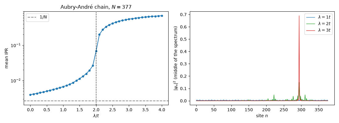
The mean IPR of a 377-site chain stays of order \(1/N\) below \(\lambda = 2t\) (rising only as the states, still extended, grow patchy near the transition) and jumps to \(O(1)\) just above it.

N = 377
lams = np.linspace(0., 4., 41)
ipr = np.array([aubry_andre(N, lam).ipr.mean() for lam in lams])
assert np.all(ipr[lams <= 1.5] < 5. / N)
assert np.all(ipr[lams >= 2.2] > 0.25)
print('mean IPR < 5/N for lambda <= 1.5 t, > 0.25 for lambda >= 2.2 t: OK')

mean IPR < 5/N for lambda <= 1.5 t, > 0.25 for lambda >= 2.2 t: OK

Unlike Anderson’s random potential

At the same strength \(\lambda = W = t\), the Anderson chain is localized (its IPR does not shrink with length) while the Aubry-André chain is extended (its IPR falls as \(1/N\)).

sizes = (144, 610)
ipr_aa = [aubry_andre(n, 1.).ipr.mean() for n in sizes]
ipr_and = [np.mean([anderson(n, 1., seed).ipr.mean() for seed in range(4)]) for n in sizes]
assert 0.7 < (ipr_aa[0] / ipr_aa[1]) / (sizes[1] / sizes[0]) < 1.3  # IPR ~ 1/N
assert ipr_and[0] / ipr_and[1] < 1.5  # IPR saturates
print('lambda = W = t: Aubry-Andre IPR ~ 1/N (extended), Anderson IPR saturates (localized): OK')

lambda = W = t: Aubry-Andre IPR ~ 1/N (extended), Anderson IPR saturates (localized): OK

Aubry’s self-duality

On a ring of \(F_n = 233\) sites with \(\beta = F_{n-1}/F_n\) (a Fibonacci approximant of the golden ratio, so the potential fits the ring), the duality is exact: the spectrum at \(\lambda\) is \(\lambda/2t\) times the spectrum at \(4t^2/\lambda\).

for lam in (0.5, 1., 1.7):
    e1 = np.sort(aubry_andre(233, lam, beta=144 / 233, phi=0., periodic=True).en.real)
    e2 = np.sort(aubry_andre(233, 4 / lam, beta=144 / 233, phi=0., periodic=True).en.real)
    assert np.allclose(e1, lam / 2 * e2, atol=1e-10)
print('spectrum(lambda) = lambda/2 * spectrum(4/lambda) on the Fibonacci ring: OK')

spectrum(lambda) = lambda/2 * spectrum(4/lambda) on the Fibonacci ring: OK

Extended, critical and localized states

fig, axes = plt.subplots(1, 2, figsize=(11, 4))
axes[0].semilogy(lams, ipr, 'o-', ms=4)
axes[0].axvline(2., c='k', ls=':')
axes[0].axhline(1 / N, c='C7', ls='--', label='$1/N$')
axes[0].set_xlabel(r'$\lambda/t$')
axes[0].set_ylabel('mean IPR')
axes[0].set_title('Aubry-André chain, $N = {}$'.format(N))
axes[0].legend()
for lam, c in ((1., 'C0'), (2., 'C2'), (3., 'C3')):
    sys = aubry_andre(N, lam)
    axes[1].plot(sys.intensity[:, N // 2], c, lw=1, label=r'$\lambda = {:g}t$'.format(lam))
axes[1].set_xlabel('site $n$')
axes[1].set_ylabel(r'$|\psi_n|^2$ (middle of the spectrum)')
axes[1].legend()
fig.tight_layout()