Anomalous Floquet Topological Phases: Edge States With Zero Chern Numbers#

In a static insulator the chiral edge states in a gap are counted by the Chern numbers of the bands below it. Kitagawa, Berg, Rudner and Demler (2010) found that a periodically driven lattice escapes this rule: since quasienergies are only defined modulo $\omega = 2\pi/T$, edge states can wind around the whole Floquet zone, and a driven system can have chiral edge states although every Floquet band has $C = 0$. Rudner, Lindner, Berg and Levin (2013) built the minimal example – a five-step drive of the bipartite square lattice in which the hopping $J$ is on along one bond direction $\mathbf{b}_s$ per step (right, up, left, down, then a pause), all under a sublattice potential $\delta_{AB} = \epsilon_A - \epsilon_B$ – and the invariant that counts these states: the winding number

\[W[U_\epsilon] = \frac{1}{8\pi^2}\int dt\,dk_x\,dk_y\, \mathrm{Tr}\left(U_\epsilon^{-1}\partial_tU_\epsilon \left[U_\epsilon^{-1}\partial_{k_x}U_\epsilon, U_\epsilon^{-1}\partial_{k_y}U_\epsilon\right]\right)\]

of the evolution $U(\mathbf{k}, t)$ over the whole period, closed by the return map $e^{iH_F^\epsilon t}$ (the branch cut of $H_F$ in the gap $\epsilon$). At “perfect transfer”, $JT/5 = \pi/2$, each step moves a particle across its bond with certainty: in the bulk it circles a plaquette and comes back, $U(T) = 1$, while on the edge a bond is missing and it moves on. Photonic lattices of coupled waveguides realized these anomalous phases (Maczewsky et al.; Mukherjee et al., both 2017).

step_drive() builds the drive, exactly, from five KSpace models (or ribbons, or real-space System flakes); winding_number() gives $W$ and edge_state_count() counts the edge states of a ribbon independently.

import numpy as np
import matplotlib.pyplot as plt

from tbkit.floquet import step_drive
from tbkit.kspace import KSpace, ribbon
from tbkit.lattice import Lattice
from tbkit.plot import Plot
from tbkit.system import System

T = 1.
omega = 2 * np.pi / T
# bipartite square lattice (bond length 1): A at (0, 0), B at (1, 0)
lat = Lattice(unit_cell=[{'tag': 'a', 'r0': (0., 0.)}, {'tag': 'b', 'r0': (1., 0.)}],
                  prim_vec=[(2., 0.), (1., 1.)])
# the bonds b_1..b_4 = right, up, left, down, from A to B, as the cell offset R of B
BONDS = [(0, 0), (-1, 1), (-1, 0), (0, -1)]

The lattice#

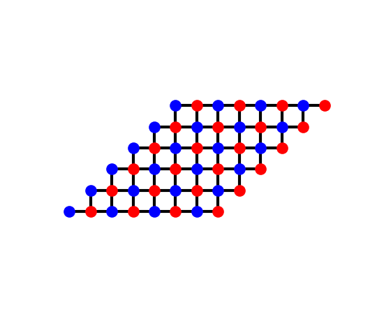
A square lattice split into its two sublattices A and B (two colours): every nearest-neighbour bond joins an A site to a B site. The drive switches the four bonds of each A site on one at a time – right, up, left, down – and leaves them all off in the fifth step.

patch = Lattice(unit_cell=lat.unit_cell, prim_vec=lat.prim_vec)
patch.get_lattice(n1=4, n2=6)
vis = System(patch)
vis.set_hopping([{'n': 1, 't': 1.}])
fig_lat = Plot(vis).lattice(plt_hop=True, ms=12, figsize=(5.5, 4.5))

The five-step drive:

def hoppings(step, J):
    return [] if step == 4 else [{'i': 0, 'j': 1, 'R': BONDS[step], 't': -J}]


def five_step(J, delta_ab=0., width=None):
    '''The drive of Rudner et al.: KSpace models, or ribbons *width* cells wide.'''
    onsite = {'a': delta_ab / 2, 'b': -delta_ab / 2}
    models = []
    for step in range(5):
        if width is None:
            ks = KSpace(lat)
            ks.set_hopping(hoppings(step, J))
            ks.set_onsite(onsite)
        else:
            ks = ribbon(lat, hoppings(step, J), width, onsite=onsite)
        models.append(ks)
    return step_drive(models, [T / 5] * 5)

Perfect transfer: trivial bands, W = 1#

$U(\mathbf{k}, T) = 1$: both Floquet bands sit at quasienergy 0, so $H_F = 0$ and every Chern number vanishes – yet the winding number in the gap at $\pi/T$ is 1.

J_perfect = 2.5 * np.pi / T  # J T/5 = pi/2
bulk = five_step(J_perfect)
quasi = bulk.mesh_bands(12)
chern = bulk.chern_number([0, 1], nk=12)
w_pi = bulk.winding_number(np.pi / T)
print('max |quasienergy| = {:.1e}, C = {:.1e}, W(pi/T) = {:.12f}'.format(np.abs(quasi).max(), chern, w_pi))
assert np.allclose(quasi, 0., atol=1e-12)
assert abs(chern) < 1e-10
assert abs(w_pi - 1.) < 1e-10

max |quasienergy| = 1.0e-15, C = 2.8e-16, W(pi/T) = 1.000000000000

The ribbon: one chiral mode per edge#

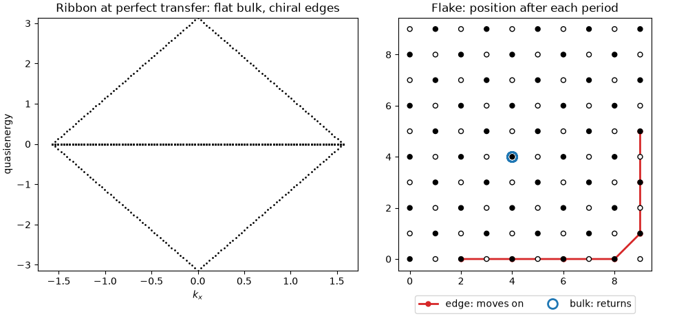
A ribbon along x (edges at the bottom and top) has two branches with $d\epsilon/dk = \pm1/T$ crossing every quasienergy. Counting the states that cross the gap at $\pi/T$, weighted by their weight on each half of the ribbon, gives +1 on the bottom edge and -1 on the top edge: $W$ in the bulk, $-W$ on the other side.

strip = five_step(J_perfect, width=10)
n_bottom, n_top = strip.edge_state_count(np.pi / T)
print('Edge states crossing pi/T: bottom {:+.6f}, top {:+.6f}'.format(n_bottom, n_top))
assert np.isclose(n_bottom, 1.) and np.isclose(n_top, -1.)

Edge states crossing pi/T: bottom +1.000000, top -1.000000

Real space: the bulk returns, the edge moves#

On a finite flake built with System (one bond direction per step, picked by angle and sublattice tags), $U(T)$ is a permutation: a particle started in the bulk is back on its site after every period, one started on the edge of sublattice A at the bottom moves right, one unit cell (two sites) per period, and around the flake counterclockwise.

flake_lat = Lattice(unit_cell=[{'tag': 'a', 'r0': (0., 0.)}, {'tag': 'b', 'r0': (1., 0.)},
                                          {'tag': 'b', 'r0': (0., 1.)}, {'tag': 'a', 'r0': (1., 1.)}],
                          prim_vec=[(2., 0.), (0., 2.)])
flake_lat.get_lattice(n1=5, n2=5)
x, y = flake_lat.coor['x'], flake_lat.coor['y']
steps = []
for ang, tag in [(0., 'ab'), (90., 'ab'), (0., 'ba'), (90., 'ba')]:  # b_1..b_4, from A to B
    sys = System(flake_lat)
    sys.set_hopping([{'n': 1, 'ang': ang, 'tag': tag, 't': -J_perfect}])
    steps.append(sys)
steps.append(np.zeros((flake_lat.sites, flake_lat.sites)))  # step 5: nothing
flake = step_drive(steps, [T / 5] * 5)


def trajectory(x0, y0, n_periods):
    psi = np.zeros(flake_lat.sites, complex)
    psi[np.where((x == x0) & (y == y0))[0][0]] = 1.
    states = flake.evolve(psi, n_periods)
    sites = np.argmax(np.abs(states), axis=1)
    assert np.allclose(np.abs(states[np.arange(len(sites)), sites]), 1.)  # on one site
    return x[sites], y[sites]


x_bulk, y_bulk = trajectory(4., 4., 6)
x_edge, y_edge = trajectory(2., 0., 6)
print('Bulk particle:', list(zip(x_bulk, y_bulk))[:3], '...')
print('Edge particle:', list(zip(x_edge, y_edge)))
assert np.all(x_bulk == 4.) and np.all(y_bulk == 4.)
assert np.array_equal(x_edge[:5], [2., 4., 6., 8., 9.]) and np.array_equal(y_edge[:5], [0., 0., 0., 0., 1.])
assert np.array_equal(x_edge[5:], [9., 9.]) and np.array_equal(y_edge[5:], [3., 5.])

fig, axes = plt.subplots(1, 2, figsize=(10, 4.6), layout='constrained')
en_strip = []
k_strip = np.linspace(-np.pi / 2, np.pi / 2, 101)  # |a1| = 2
for k in k_strip:
    en_strip.append(np.linalg.eigvalsh(strip.get_ham([k])))
axes[0].plot(k_strip, np.array(en_strip), 'k.', ms=2)
axes[0].set_xlabel(r'$k_x$')
axes[0].set_ylabel('quasienergy')
axes[0].set_ylim(-np.pi / T, np.pi / T)
axes[0].set_title('Ribbon at perfect transfer: flat bulk, chiral edges')
axes[1].scatter(x, y, c=np.where(flake_lat.coor['tag'] == 'a', 'k', 'w'), edgecolors='k', s=25, zorder=3)
axes[1].plot(x_edge, y_edge, '-o', color='C3', lw=2, ms=5, label='edge: moves on')
axes[1].plot(x_bulk, y_bulk, 'o', color='C0', ms=10, mfc='none', mew=2, label='bulk: returns')
axes[1].set_aspect('equal')
axes[1].set_title('Flake: position after each period')
axes[1].legend(loc='upper center', bbox_to_anchor=(0.5, -0.08), ncol=2)

Ribbon at perfect transfer: flat bulk, chiral edges, Flake: position after each period

Bulk particle: [(np.float64(4.0), np.float64(4.0)), (np.float64(4.0), np.float64(4.0)), (np.float64(4.0), np.float64(4.0))] ...
Edge particle: [(np.float64(2.0), np.float64(0.0)), (np.float64(4.0), np.float64(0.0)), (np.float64(6.0), np.float64(0.0)), (np.float64(8.0), np.float64(0.0)), (np.float64(9.0), np.float64(1.0)), (np.float64(9.0), np.float64(3.0)), (np.float64(9.0), np.float64(5.0))]

<matplotlib.legend.Legend object at 0x10f312f90>

Away from perfect transfer: the phase diagram#

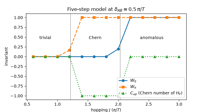
Along the cut $\delta_{AB} = 0.5\,\pi/T$ of the paper’s Fig. 3d, the winding numbers $W_0, W_\pi$ in the gaps at 0 and $\pi/T$, and the Chern number of the upper Floquet band. The anomalous phase ($W_0 = W_\pi = 1$, $C = 0$) survives from perfect transfer down to the closing of the gap at 0, at $J = 2.03\,\pi/T$; the Chern-insulating phase ($W_\pi = 1$, $C_{up} = -1$ with tbkit’s sign, $\mathcal{C} = +1$ with the paper’s) lies between it and the closing of the gap at $\pi/T$, $J = 1.21\,\pi/T$; below is the trivial phase. The paper reads the two boundaries as roughly 1.3 and 2.1 off its figure. Across the upper band, $W_\pi - W_0 = -C_{up}$ everywhere, as it must. Next to a gap closing the raw $W$ is not yet an integer at the default k-grid ($W_0 = 0.2$ at $J = 2.0\,\pi/T$, 0.03 from the closing): such points are left out of the checks, as the tolerance of winding_number prescribes.

The static rule “edge states in a gap = minus the total Chern number of the bands below” (tbkit’s sign, see winding_number) would give $-C_{low}$ at 0 and 0 at $\pi/T$ (where the whole zone is below). It fails in both non-trivial phases.

delta_ab = 0.5 * np.pi / T
Js = np.arange(0.6, 3.01, 0.2) * np.pi / T
w0, wpi, c_up = [], [], []
for J in Js:
    drive = five_step(J, delta_ab)
    w0.append(drive.winding_number(0.))
    wpi.append(drive.winding_number(np.pi / T))
    c_up.append(drive.chern_number(1, nk=16))
w0, wpi, c_up = np.array(w0), np.array(wpi), np.array(c_up)
jn = Js * T / np.pi
print('J (pi/T) :', np.round(jn, 1))
print('W_0      :', np.round(w0, 3))
print('W_pi     :', np.round(wpi, 3))
print('C_up     :', np.round(c_up, 3))
clear = (np.abs(jn - 1.21) > 0.15) & (np.abs(jn - 2.03) > 0.15)  # away from the gap closings
assert np.allclose(w0[clear], np.round(w0[clear]), atol=1e-2)
assert np.allclose(wpi[clear], np.round(wpi[clear]), atol=1e-2)
assert np.allclose(c_up, np.round(c_up), atol=1e-6)
assert np.allclose((wpi - w0)[clear], -c_up[clear], atol=1e-2)
trivial, chern_phase, anomalous = jn < 1.21, (jn > 1.21) & (jn < 2.03), jn > 2.03
assert np.allclose(np.round(w0[trivial]), 0) and np.allclose(np.round(wpi[trivial]), 0)
assert np.allclose(np.round(w0[chern_phase & clear]), 0) and np.allclose(np.round(wpi[chern_phase & clear]), 1)
assert np.allclose(np.round(c_up[chern_phase]), -1)
assert np.allclose(np.round(w0[anomalous & clear]), 1) and np.allclose(np.round(wpi[anomalous]), 1)
assert np.allclose(np.round(c_up[anomalous]), 0)
# where the Chern numbers fail: the static rule misses W in the non-trivial phases
static_rule_0 = -(-c_up)  # -C_low, with C_low = -C_up
fails = clear & ((np.round(w0) != np.round(static_rule_0)) | (np.round(wpi) != 0))
print('The Chern numbers of H_F miss the edge states at J (pi/T) =', np.round(jn[fails], 1))
assert np.all(fails[clear] == (jn[clear] > 1.21))

J (pi/T) : [0.6 0.8 1.  1.2 1.4 1.6 1.8 2.  2.2 2.4 2.6 2.8 3. ]
W_0      : [0.000e+00 0.000e+00 0.000e+00 0.000e+00 0.000e+00 0.000e+00 1.000e-03
 1.950e-01 1.000e+00 1.000e+00 1.000e+00 1.000e+00 1.004e+00]
W_pi     : [ 0.    -0.     0.     0.167  1.     1.     1.     1.     1.     1.
  1.     1.     1.   ]
C_up     : [ 0.  0. -0. -0. -1. -1. -1. -1.  0.  0.  0. -0.  0.]
The Chern numbers of H_F miss the edge states at J (pi/T) = [1.4 1.6 1.8 2.2 2.4 2.6 2.8 3. ]

The ribbon agrees gap by gap#

In the anomalous phase (both Chern numbers zero) the ribbon has chiral states in both gaps; in the Chern phase only at $\pi/T$.

for J, expected in [(1.6 * np.pi / T, (0, 1)), (2.4 * np.pi / T, (1, 1))]:
    rib = five_step(J, delta_ab, width=20)
    counts = [rib.edge_state_count(eps)[0] for eps in (0., np.pi / T)]
    print('J = {:.1f} pi/T: bottom-edge states at 0 and pi/T: {:+.4f} {:+.4f}'.format(J * T / np.pi, *counts))
    assert np.allclose(counts, expected, atol=1e-3)

fig, ax = plt.subplots(figsize=(7, 3.8))
ax.plot(jn, w0, 'o-', color='C0', lw=2, label=r'$W_0$')
ax.plot(jn, wpi, 's--', color='C1', lw=2, label=r'$W_\pi$')
ax.plot(jn, c_up, '^:', color='C2', lw=2, label=r'$C_{up}$ (Chern number of $H_F$)')
for jc in (1.21, 2.03):
    ax.axvline(jc, color='grey', lw=0.8)
ax.text(0.8, 0.45, 'trivial', ha='center')
ax.text(1.62, 0.45, 'Chern', ha='center')
ax.text(2.55, 0.45, 'anomalous', ha='center')
ax.set_xlabel(r'hopping $J$ ($\pi/T$)')
ax.set_ylabel('invariant')
ax.set_title(r'Five-step model at $\delta_{AB} = 0.5\,\pi/T$')
ax.legend(loc='lower right')

$Five-step model at $\delta_{AB} = 0.5\,\pi/T$$

J = 1.6 pi/T: bottom-edge states at 0 and pi/T: +0.0000 +1.0000
J = 2.4 pi/T: bottom-edge states at 0 and pi/T: +1.0000 +1.0000

<matplotlib.legend.Legend object at 0x10f0a8590>

Total running time of the script: (0 minutes 4.223 seconds)

Gallery generated by Sphinx-Gallery