Brillouin Zones and Standard High-Symmetry Paths

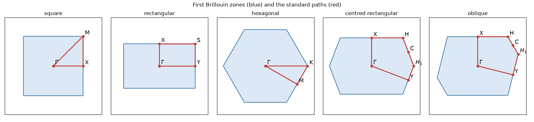
L. Brillouin (1930) gave the zone that carries his name: the set of \(\mathbf{k}\) closer to the origin than to any other reciprocal lattice vector \(\mathbf{G}\), the Wigner-Seitz cell of the reciprocal lattice. Its faces are the planes where Bragg reflection \(|\mathbf{k}| = |\mathbf{k} - \mathbf{G}|\) opens band gaps, and its corners and face centres are the points of highest symmetry, where bands reach their extrema, cross or are degenerate. A band structure is therefore drawn along a path through them. W. Setyawan and S. Curtarolo (2010) fixed one standard path per Bravais lattice, so that band structures from different codes can be compared at a glance.

tbkit.kspace.high_symmetry_path() recognizes the Bravais lattice from the primitive vectors, whatever their choice and orientation, and returns the standard path; tbkit.kspace.cubic_path() builds any path of a cubic crystal from the tables of high-symmetry points. This example checks that every point it returns lies on the zone boundary, that the path does not depend on the choice of primitive vectors, and that the s-band of the fcc and bcc lattices takes its closed-form values at the labelled points.

from itertools import product

import numpy as np
import matplotlib.pyplot as plt

from tbkit.lattice import Lattice
from tbkit.kspace import KSpace, cubic_path, high_symmetry_path, reciprocal_vectors
from tbkit.plot import Plot
from tbkit.system import System


def lattice_2d(prim_vec):
    return Lattice(unit_cell=[{'tag': 'a', 'r0': (0., 0.)}], prim_vec=prim_vec)


def zone_check(points, prim_vec):
    '''
    For each k-point: is it in the closed Wigner-Seitz cell (no G closer
    than the origin), and on its boundary (some G exactly as close)?
    '''
    rec = np.array(reciprocal_vectors(prim_vec))
    gs = np.array([n @ rec for n in product(range(-3, 4), repeat=2) if any(n)])
    inside, boundary = [], []
    for k in points:
        d0, dg = k @ k, np.sum((k - gs) ** 2, axis=1)
        inside.append(bool(np.all(d0 <= dg + 1e-9)))
        boundary.append(bool(np.any(np.isclose(d0, dg))))
    return inside, boundary

The five 2D Bravais lattices

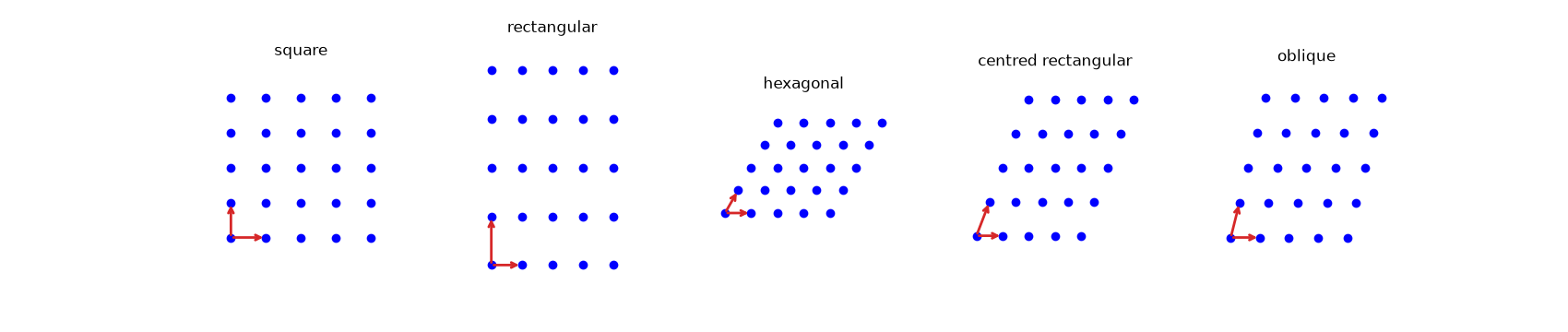
Square, rectangular, hexagonal, centred rectangular and oblique. Each path starts and ends at \(\Gamma\). Every other point is on the boundary of the zone: equidistant from \(\Gamma\) and from at least one other reciprocal lattice vector, and closer to \(\Gamma\) than to any. The oblique lattice has no symmetry beyond inversion, so its path follows the edges of half the zone (\(X, H, C, H_1, Y\)).

s3 = np.sqrt(3.)
bravais = {'square': [(1., 0.), (0., 1.)],
           'rectangular': [(1., 0.), (0., 1.6)],
           'hexagonal': [(1., 0.), (0.5, s3 / 2)],
           'centred rectangular': [(1., 0.), (0.5, 1.3)],
           'oblique': [(1., 0.), (0.3, 1.2)]}

# The five lattices in real space, with their primitive vectors
# :math:`\mathbf{a}_1` and :math:`\mathbf{a}_2` (arrows):
fig_lat, axes = plt.subplots(1, 5, figsize=(17, 3.6))
for ax, (name, prim_vec) in zip(axes, bravais.items()):
    patch = lattice_2d(prim_vec)
    patch.get_lattice(n1=5, n2=5)
    Plot(System(patch)).lattice(ms=7, ax=ax)
    for a in prim_vec:
        ax.annotate('', xy=a, xytext=(0., 0.), arrowprops=dict(arrowstyle='->', color='C3', lw=2))
    ax.set_title(name)

Their Brillouin zones and high-symmetry paths:

fig_bz, axes = plt.subplots(1, 5, figsize=(17, 3.9))
for ax, (name, prim_vec) in zip(axes, bravais.items()):
    points, labels = high_symmetry_path(lattice_2d(prim_vec))
    inside, boundary = zone_check(points, prim_vec)
    print('{:<20} {:<36} on the boundary: {}'.format(
        name, ' '.join(lab.strip('$').replace('\\', '') for lab in labels), boundary))
    assert all(inside)
    assert not boundary[0] and not boundary[-1]       # Gamma, the centre
    assert all(boundary[1:-1])
    # draw the zone: the Bragg planes of the nearest reciprocal vectors
    rec = np.array(reciprocal_vectors(prim_vec))
    kmax = 1.15 * max(np.linalg.norm(p) for p in points)
    kx = np.linspace(-kmax, kmax, 401)
    kxx, kyy = np.meshgrid(kx, kx)
    kk = np.stack([kxx, kyy], axis=-1)
    gs = np.array([n @ rec for n in product(range(-2, 3), repeat=2) if any(n)])
    margin = np.min(np.sum((kk[..., None, :] - gs) ** 2, axis=-1), axis=-1) - np.sum(kk ** 2, axis=-1)
    ax.contourf(kxx, kyy, margin, levels=[0., np.inf], colors=['#dce8f5'])
    ax.contour(kxx, kyy, margin, levels=[0.], colors='#3b76af')
    path = np.array(points)
    ax.plot(path[:, 0], path[:, 1], 'o-', color='#c53a32', lw=2, ms=5)
    for p, lab in zip(points[:-1], labels[:-1]):
        ax.annotate(lab, p, textcoords='offset points', xytext=(4, 4), fontsize=13)
    ax.set_aspect('equal')
    ax.set_xticks([])
    ax.set_yticks([])
    ax.set_title(name)
fig_bz.suptitle('First Brillouin zones (blue) and the standard paths (red)')
fig_bz.tight_layout()

square               Gamma X M Gamma                      on the boundary: [False, True, True, False]
rectangular          Gamma X S Y Gamma                    on the boundary: [False, True, True, True, False]
hexagonal            Gamma M K Gamma                      on the boundary: [False, True, True, False]
centred rectangular  Gamma X H C H_1 Y Gamma              on the boundary: [False, True, True, True, True, True, False]
oblique              Gamma X H C H_1 Y Gamma              on the boundary: [False, True, True, True, True, True, False]

The path does not depend on the primitive vectors

\((\mathbf{a}_1, \mathbf{a}_2)\) and \((\mathbf{a}_1, \mathbf{a}_1 + \mathbf{a}_2)\) span the same triangular lattice, and so does any rotation of them. The Bravais lattice is recognized from a reduced basis, so the three give the same \(M\) and \(K\), at \(|M| = 2\pi/(\sqrt3 a)\) and \(|K| = 4\pi/(3a)\) from \(\Gamma\).

a1, a2 = np.array([1., 0.]), np.array([0.5, s3 / 2])
rot = np.array([[np.cos(0.3), -np.sin(0.3)], [np.sin(0.3), np.cos(0.3)]])
for basis in ([a1, a2], [a1, a1 + a2], [rot @ a1, rot @ a2]):
    points, labels = high_symmetry_path(lattice_2d([tuple(v) for v in basis]))
    assert labels == [r'$\Gamma$', 'M', 'K', r'$\Gamma$']
    assert np.isclose(np.linalg.norm(points[1]), 2 * np.pi / s3)
    assert np.isclose(np.linalg.norm(points[2]), 4 * np.pi / 3)
print('|M| = 2 pi/(sqrt3 a) and |K| = 4 pi/(3a) for three bases of the triangular lattice.')

|M| = 2 pi/(sqrt3 a) and |K| = 4 pi/(3a) for three bases of the triangular lattice.

fcc and bcc: the s band at the labelled points

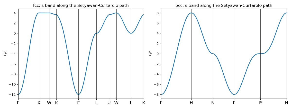
One s orbital per site with nearest-neighbour hopping \(-t\). On the fcc lattice (12 neighbours at \(a/\sqrt2\)),

\[E(\mathbf{k}) = -4t\left[\cos\tfrac{k_xa}{2}\cos\tfrac{k_ya}{2} + \cos\tfrac{k_ya}{2}\cos\tfrac{k_za}{2} + \cos\tfrac{k_za}{2}\cos\tfrac{k_xa}{2}\right],\]

so \(E(\Gamma) = -12t\), \(E(X) = E(W) = 4t\), \(E(L) = 0\) and \(E(K) = E(U) = (4\sqrt2 - 2)t\). On the bcc lattice (8 neighbours at \(\sqrt3a/2\)), \(E = -8t\cos\tfrac{k_xa}{2}\cos\tfrac{k_ya}{2}\cos\tfrac{k_za}{2}\): \(-8t\) at \(\Gamma\), \(+8t\) at \(H\), and 0 at \(N\) and \(P\). The primitive vectors given here are not the conventional cubic axes; the path is found anyway.

a, t = 1., 1.
cells = {'fcc': [(0., a/2, a/2), (a/2, 0., a/2), (a/2, a/2, 0.)],
         'bcc': [(-a/2, a/2, a/2), (a/2, -a/2, a/2), (a/2, a/2, -a/2)]}
expected = {'fcc': {r'$\Gamma$': -12., 'X': 4., 'W': 4., 'L': 0., 'K': 4 * np.sqrt(2.) - 2,
                    'U': 4 * np.sqrt(2.) - 2},
            'bcc': {r'$\Gamma$': -8., 'H': 8., 'N': 0., 'P': 0.}}

fig_3d, axes = plt.subplots(1, 2, figsize=(12, 4.5))
for ax, (name, prim_vec) in zip(axes, cells.items()):
    lat = Lattice(unit_cell=[{'tag': 'a', 'r0': (0., 0., 0.)}], prim_vec=prim_vec)
    ks = KSpace(lat)
    ks.set_hopping([{'n': 1, 't': -t}])
    points, labels = high_symmetry_path(lat)
    energies = ks.get_bands(np.array(points))[:, 0]
    for lab, e in zip(labels, energies):
        assert np.isclose(e, expected[name][lab] * t, atol=1e-12), (name, lab, e)
    print('{}: {}'.format(name, ', '.join('E({}) = {:+.4f}'.format(
        lab.strip('$').replace('\\', ''), e) for lab, e in zip(labels, energies))))
    dist, en = ks.k_path(points, nk=60)
    ax.plot(dist, en[:, 0], lw=2)
    for node in ks.nodes:
        ax.axvline(node, color='k', lw=0.5)
    ax.set_xticks(ks.nodes)
    ax.set_xticklabels(labels, fontsize=13)
    ax.set_xlim(dist[0], dist[-1])
    ax.set_ylabel('$E/t$')
    ax.set_title('{}: s band along the Setyawan-Curtarolo path'.format(name))
fig_3d.tight_layout()

fcc: E(Gamma) = -12.0000, E(X) = +4.0000, E(W) = +4.0000, E(K) = +3.6569, E(Gamma) = -12.0000, E(L) = +0.0000, E(U) = +3.6569, E(W) = +4.0000, E(L) = +0.0000, E(K) = +3.6569
bcc: E(Gamma) = -8.0000, E(H) = +8.0000, E(N) = +0.0000, E(Gamma) = -8.0000, E(P) = -0.0000, E(H) = +8.0000

Other paths of cubic crystals

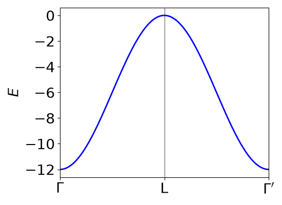
Tables give the high-symmetry points of cubic crystals in units of \(2\pi/a\) along the cubic axes, \(a\) the side of the conventional cube. cubic_path() turns them into k-points. From the Setyawan-Curtarolo table of the fcc lattice it rebuilds the path of high_symmetry_path. Any other path follows from the same points, e.g. along the whole cube diagonal: the s band of fcc rises from \(-12t\) at \(\Gamma\) to 0 at \(L\) and comes back to \(-12t\) at \((1, 1, 1)\,2\pi/a\), a reciprocal lattice vector of fcc (\(L\) is the midpoint of the hexagonal face it bisects), so an image of \(\Gamma\).

G = r'$\Gamma$'
fcc_table = {G: (0, 0, 0), 'X': (0, 1, 0), 'W': (.5, 1, 0), 'K': (.75, .75, 0),
             'L': (.5, .5, .5), 'U': (.25, 1, .25), r"$\Gamma'$": (1, 1, 1)}
fcc_lat = Lattice(unit_cell=[{'tag': 'a', 'r0': (0., 0., 0.)}], prim_vec=cells['fcc'])
standard, names = high_symmetry_path(fcc_lat)
rebuilt, _ = cubic_path(fcc_table, names, a=a)
assert np.allclose(np.array(rebuilt), np.array(standard))
print('cubic_path rebuilds the fcc path from its table of points.')

fcc = KSpace(fcc_lat)
fcc.set_hopping([{'n': 1, 't': -t}])
diagonal, labels = cubic_path(fcc_table, [G, 'L', r"$\Gamma'$"], a=a)
e_diag = fcc.get_bands(np.array(diagonal))[:, 0]
assert np.allclose(e_diag, [-12. * t, 0., -12. * t])
dist, en = fcc.k_path(diagonal, nk=60)
fig_diag = fcc.plot_bands(node_labels=labels, figsize=(5.5, 4.))

cubic_path rebuilds the fcc path from its table of points.