The Intrinsic Thermal Hall Effect and the Wiedemann-Franz Law

A temperature gradient also drives a transverse heat current, \(j^Q_x = \kappa_{xy}(-\partial_yT)\). Computing it from the Kubo formula is subtle: part of the heat current circulates as a bound magnetization current and does not flow. Qin, Niu and Shi (2011) subtracted it and found the intrinsic electronic thermal Hall conductivity as one more weighted integral of the Berry curvature,

\[\kappa_{xy} = \frac{k_B^2T}{h}\,\frac{1}{2\pi}\int_{BZ}d^2k\sum_nc_2(x_n)\,\Omega_n\, , \qquad c_2(x) = \int_x^\infty y^2\left(-\frac{\partial f}{\partial y}\right)dy\, ,\]

\(x_n = (E_n-\mu)/k_BT\). Equivalently, \(\kappa_{xy} = \frac{1}{e^2T}\int dE\,(E-\mu)^2(-\partial f/\partial E)\,\sigma_{xy}(E)\). At low temperature only \(c_2(-\infty) = \pi^2/3\) matters, and \(\kappa_{xy}\) and \(\sigma_{xy}\) obey the Wiedemann-Franz law

\[\frac{\kappa_{xy}}{T\sigma_{xy}} = \frac{\pi^2}{3}\frac{k_B^2}{e^2}\, :\]

in a Chern insulator the thermal Hall conductance is quantized, \(\kappa_{xy}/T = C\,\pi^2k_B^2/3h\), as the heat carried by its chiral edge states.

thermal_hall_conductivity() evaluates it for the Haldane model below.

import numpy as np
import matplotlib.pyplot as plt
from scipy.integrate import trapezoid

import tbkit.lattices as lattices
from tbkit.bridges import finite_system
from tbkit.kspace import KSpace
from tbkit.plot import Plot


def haldane(M, t2=0.2):
    '''Haldane model: nearest-neighbour t = 1, i t2 on the second neighbours, mass +-M.'''
    hal = KSpace(lattices.honeycomb())
    hal.set_hopping([{'i': 0, 'j': 1, 'R': R, 't': 1.} for R in [(0, 0), (-1, 0), (0, -1)]])
    for R in [(0, 1), (-1, 0), (1, -1)]:
        hal.set_hopping([{'i': 0, 'j': 0, 'R': R, 't': 1j*t2}, {'i': 1, 'j': 1, 'R': R, 't': -1j*t2}])
    hal.set_onsite({'a': M, 'b': -M})
    return hal


hal = haldane(0.3)

The lattice

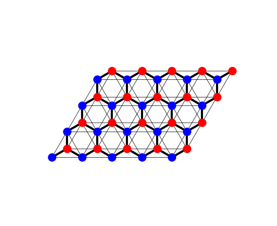
The Haldane model on a patch of \(5\times4\) cells (finite_system()), each bond drawn with a width proportional to its amplitude: the honeycomb lattice’s two sublattices (‘a’ and ‘b’, in two colours), the nearest-neighbour hopping \(t\) (thick) and the complex second-neighbour hoppings \(\pm it_2\) within each sublattice (thin), which break time-reversal symmetry.

fig_lat = Plot(finite_system(haldane(0.3), (5, 4))).lattice(plt_hop=True, ms=12, figsize=(5.5, 4.5))

The Wiedemann-Franz ratio across the spectrum

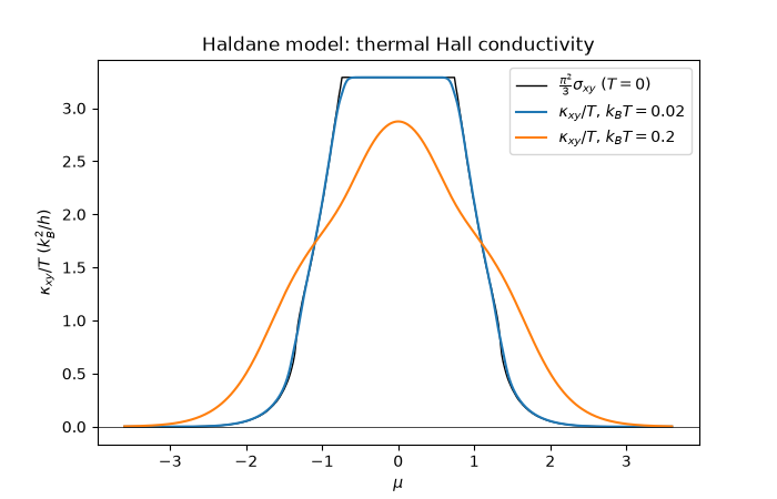
\(\kappa_{xy}/T\) (in \(k_B^2/h\)) next to \(\frac{\pi^2}{3}\sigma_{xy}\) (\(\sigma_{xy}\) in \(e^2/h\)): on the plateau they are equal, \(\pi^2/3\) for \(C = 1\).

mu = np.linspace(-3.6, 3.6, 361)
sigma = hal.hall_conductivity(mu, nk=120)
temps = (0.02, 0.2)
kappa = {T: hal.thermal_hall_conductivity(mu, T, nk=120) for T in temps}

gap = np.abs(mu) < 0.2
plateau = kappa[0.02][gap] / 0.02
print('T = 0.02: kappa/T in the gap from {:.8f} to {:.8f} (pi^2/3 = {:.8f})'.format(
    plateau.min(), plateau.max(), np.pi ** 2 / 3))
assert np.allclose(plateau, np.pi ** 2 / 3, atol=1e-6)
assert abs(hal.thermal_hall_conductivity(12., 0.2, nk=60)) < 1e-10  # full bands

T = 0.02: kappa/T in the gap from 3.28986813 to 3.28986813 (pi^2/3 = 3.28986813)

The law needs \(\sigma_{xy}(E)\) to vary slowly within \(k_BT\) of \(\mu\). At \(k_BT = 0.2\), comparable to the gap, the thermal window reaches the bands and the ratio drops to 0.87 in the middle of the gap. The exact relation to \(\sigma_{xy}(E)\) holds everywhere, as a fine energy grid of the \(T = 0\) Hall conductivity confirms.

e = np.linspace(-4., 4., 4001)
sigma_e = hal.hall_conductivity(e, nk=120)
for T in temps:
    x = np.abs(e[:, None] - mu[None, :]) / T
    window = np.exp(-x) / (1 + np.exp(-x)) ** 2 / T
    exact = trapezoid((e[:, None] - mu) ** 2 * window * sigma_e[:, None], e, axis=0) / T
    err = np.max(np.abs(kappa[T] - exact))
    print('T = {}: max |kappa - integral of sigma_xy(E)| = {:.1e}'.format(T, err))
    assert err < 5e-4
wf_gap = kappa[0.2][gap][len(gap[gap]) // 2] / 0.2 / (np.pi ** 2 / 3)
print('T = 0.2: kappa / (pi^2/3 T sigma) at mu = 0: {:.3f}'.format(wf_gap))
assert 0.85 < wf_gap < 0.9

fig, ax = plt.subplots(figsize=(7, 4.5))
ax.plot(mu, np.pi ** 2 / 3 * sigma, 'k', lw=1, label=r'$\frac{\pi^2}{3}\sigma_{xy}$ ($T = 0$)')
for T in temps:
    ax.plot(mu, kappa[T] / T, label=r'$\kappa_{{xy}}/T$, $k_BT = {}$'.format(T))
ax.axhline(0., color='k', lw=0.5)
ax.set_xlabel(r'$\mu$')
ax.set_ylabel(r'$\kappa_{xy}/T$ ($k_B^2/h$)')
ax.set_title('Haldane model: thermal Hall conductivity')
ax.legend()

T = 0.02: max |kappa - integral of sigma_xy(E)| = 5.8e-06
T = 0.2: max |kappa - integral of sigma_xy(E)| = 4.5e-06
T = 0.2: kappa / (pi^2/3 T sigma) at mu = 0: 0.874

<matplotlib.legend.Legend object at 0x10f25acf0>