Maximally Localized Wannier Functions: Projection and Spread Minimization

The Wannier functions of a band are the Fourier transforms of its Bloch states,

\[|n\mathbf{R}\rangle = \frac{1}{N}\sum_{\mathbf{k}} e^{-i\mathbf{k}\cdot\mathbf{R}} \sum_m U_{mn}(\mathbf{k})\,|\psi_{m\mathbf{k}}\rangle\, ,\]

and they depend on the gauge \(U(\mathbf{k})\), a unitary mixing of the bands at each k. N. Marzari and D. Vanderbilt (1997) chose the gauge that minimizes the total spread

\[\Omega = \sum_n \langle r^2\rangle_n - |\bar{\mathbf{r}}_n|^2 = \Omega_I + \tilde\Omega_D + \tilde\Omega_{OD}\, ,\]

where \(\Omega_I\) does not depend on the gauge at all: it is a property of the band group, and a lower bound on the spread.

tbkit.wannier.wannierize() follows their recipe. It first projects the Bloch states onto trial orbitals and orthonormalizes them (Lowdin), then lowers \(\tilde\Omega_D + \tilde\Omega_{OD}\) by conjugate gradients, from the overlaps of the Bloch states at neighbouring points of the k-mesh. The Wannier functions come out on the \(N_1\times N_2\) cells of the mesh, as amplitudes on the sites of a finite System.

import numpy as np
import matplotlib.pyplot as plt

import tbkit.lattices as lattices
from tbkit.bridges import finite_system
from tbkit.kspace import KSpace
from tbkit.lattice import Lattice
from tbkit.plot import Plot
from tbkit.wannier import wannierize

The SSH chain: down to the gauge-invariant bound

One band in 1D: the minimization removes \(\tilde\Omega_D\) and \(\tilde\Omega_{OD}\) entirely, so \(\Omega = \Omega_I\), and the centre is the Wilson-loop centre of wannier_centers() – the middle of the strong bond, at 0.75.

lat = Lattice(unit_cell=[{'tag': 'a', 'r0': (0., 0.)}, {'tag': 'b', 'r0': (0.5, 0.)}],
                    prim_vec=[(1., 0.)])
ssh = KSpace(lat)
ssh.set_hopping([{'i': 0, 'j': 1, 'R': (0,), 't': 0.5}, {'i': 1, 'j': 0, 'R': (1,), 't': 1.}])

Eight cells of the chain (finite_system()), orbitals a and b in two colours, bond widths proportional to the hoppings: weak (0.5) inside each cell, strong (1) between cells.

fig_lat = Plot(finite_system(ssh, 8)).lattice(plt_hop=True, ms=7, c=4., figsize=(7, 1.2))

Projection, then minimization:

nk = 20
projected = wannierize(ssh, 0, trial=[0], nk=nk, max_iter=0)  # projection only
mlwf = wannierize(ssh, 0, trial=[0], nk=nk)
print('projected: Omega = {:.5f}'.format(projected.omega))
print('MLWF:      Omega = {:.5f} after {} steps, Omega_I = {:.5f}, Omega_D = {:.1e}, Omega_OD = {:.1e}'
       .format(mlwf.omega, len(mlwf.history) - 1, mlwf.omega_i, mlwf.omega_d, mlwf.omega_od))
print('centre {:.6f} (mod 1), Wilson loop {:.6f}'.format(mlwf.centers[0, 0] % 1, ssh.wannier_centers(0, nk=nk)[0]))
assert mlwf.converged and np.all(np.diff(mlwf.history) <= 0.)
assert np.isclose(projected.omega_i, mlwf.omega_i)  # gauge invariant
assert projected.omega > mlwf.omega + 0.03
assert np.isclose(mlwf.omega, mlwf.omega_i, atol=1e-7) and mlwf.omega_d < 1e-7 and mlwf.omega_od == 0.
assert np.isclose(mlwf.centers[0, 0] % 1, 0.75) and np.isclose(ssh.wannier_centers(0, nk=nk)[0], 0.75)

projected: Omega = 0.14322
MLWF:      Omega = 0.10230 after 71 steps, Omega_I = 0.10230, Omega_D = 4.0e-12, Omega_OD = 0.0e+00
centre 0.750000 (mod 1), Wilson loop 0.750000

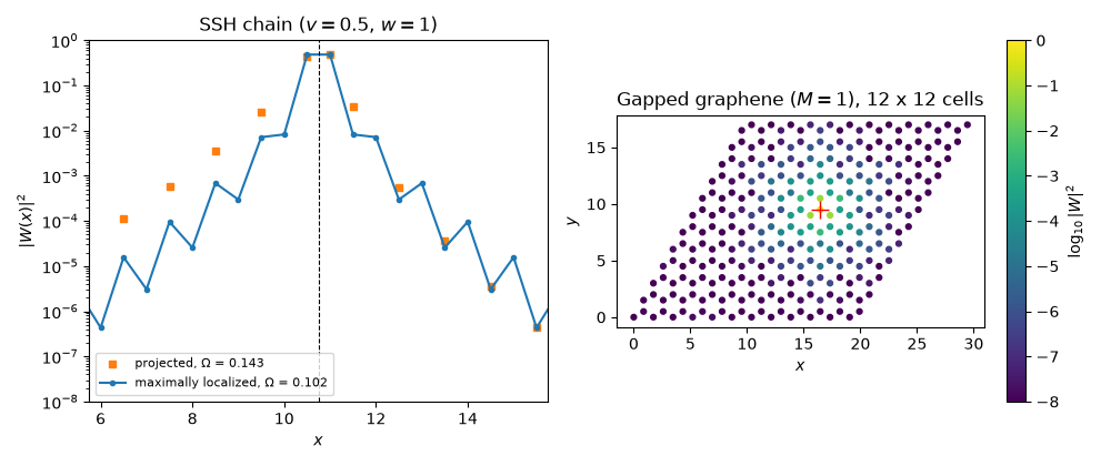
The functions themselves: the projection onto orbital a starts there, with a tail along the chain; the minimization moves the weight onto the strong bond, symmetric about its middle.

x = mlwf.positions[:, 0]
p0, p1 = np.abs(projected.functions[0]) ** 2, np.abs(mlwf.functions[0]) ** 2
c = mlwf.centers[0, 0]
assert np.isclose(p1.sum(), 1.) and np.isclose(p1 @ x, c, atol=1e-6)
d = (x - c + nk / 2) % nk - nk / 2  # distance to the centre, around the ring of nk cells
assert np.allclose(p1[np.argsort(d)], p1[np.argsort(-d)], atol=1e-5)  # mirror symmetric about the bond centre

Gapped graphene: a Wannier function on a honeycomb site

Graphene with a staggered potential \(\pm M\) (as in hexagonal boron nitride) has a trivial lower band, mostly on the low-energy sublattice b. Projected on that orbital and minimized, it gives a Wannier function centred on a b site (by threefold symmetry), whose diagonal matrix element is the band’s average energy \(\langle 0|H|0\rangle = \frac{1}{N}\sum_{\mathbf{k}}E(\mathbf{k})\).

M = 1.
bn = KSpace(lattices.honeycomb())
bn.set_hopping([{'i': 0, 'j': 1, 'R': R, 't': -1.} for R in [(0, 0), (-1, 0), (0, -1)]])
bn.set_onsite({'a': M, 'b': -M})

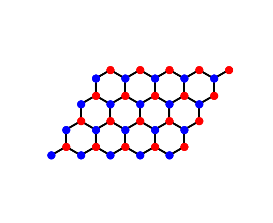
The honeycomb lattice on a patch of \(5\times4\) cells (finite_system()), sublattices a (onsite \(+M\)) and b (\(-M\)) in two colours, with the nearest-neighbour bonds.

fig_lat = Plot(finite_system(bn, (5, 4))).lattice(plt_hop=True, ms=12, figsize=(5.5, 4.5))

The Wannier function of the lower band, from a trial orbital on b:

nk = 12
wf = wannierize(bn, 0, trial=[1], nk=nk)
sites_b = wf.positions[1::2]
print('centre {} on a b site: {}'.format(wf.centers[0].round(6), np.min(np.linalg.norm(sites_b - wf.centers[0], axis=1)) < 1e-8))
print('Omega = {:.5f}, Omega_I = {:.5f}'.format(wf.omega, wf.omega_i))
assert wf.converged and wf.omega_i <= wf.omega
assert np.min(np.linalg.norm(sites_b - wf.centers[0], axis=1)) < 1e-8
torus = bn.finite_ham((nk, nk), periodic=True)
e_wf = (wf.functions[0].conj() @ torus @ wf.functions[0]).real
e_mean = bn.mesh_bands(nk)[:, 0].mean()
print('<0|H|0> = {:.10f}, mean band energy = {:.10f}'.format(e_wf, e_mean))
assert np.isclose(e_wf, e_mean, atol=1e-12)

centre [16.454483  9.5     ] on a b site: True
Omega = 0.25940, Omega_I = 0.23693
<0|H|0> = -1.9100645560, mean band energy = -1.9100645560

Plots: the SSH Wannier function before and after the minimization, and the gapped-graphene one on the sites of its finite System (wf.system).

fig, (ax1, ax2) = plt.subplots(1, 2, figsize=(10, 4.2))
order = np.argsort(x)
ax1.semilogy(x[order], p0[order], 's', ms=4, color='C1',  # zero on every a site but its own
                    label=r'projected, $\Omega$ = {:.3f}'.format(projected.omega))
ax1.semilogy(x[order], p1[order], 'o-', ms=3, color='C0', label=r'maximally localized, $\Omega$ = {:.3f}'.format(mlwf.omega))
ax1.axvline(c, color='k', lw=0.8, ls='--')
ax1.set_xlim(c - 5, c + 5)
ax1.set_ylim(1e-8, 1)
ax1.set_xlabel('$x$')
ax1.set_ylabel(r'$|W(x)|^2$')
ax1.set_title('SSH chain ($v = 0.5$, $w = 1$)')
ax1.legend(fontsize=8)

coor = wf.system.lat.coor
amp = np.abs(wf.functions[0]) ** 2
sc = ax2.scatter(coor['x'], coor['y'], c=np.log10(amp + 1e-16), s=12, cmap='viridis', vmin=-8, vmax=0)
ax2.plot(*wf.centers[0], 'r+', ms=12)
ax2.set_aspect('equal')
ax2.set_xlabel('$x$')
ax2.set_ylabel('$y$')
ax2.set_title('Gapped graphene ($M = 1$), {0} x {0} cells'.format(nk))
fig.colorbar(sc, ax=ax2, label=r'$\log_{10}|W|^2$')
fig.set_layout_engine('tight')
plt.show()